Backtransform coefficients of a Gamma-log GLMM

Question

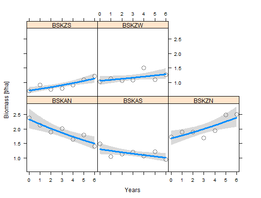
I am analysing data from an exclosure experiment, this means for several years, goats were kept outside a fence and inside the fence, plants could grow without being grazed. Outside the fence, grazing continued as usual.

Now I fitted a GLM model containing biomass in tons/ha per site over several years. As biomass should not be equal to or smaller than zero, I choose the Gamma distribution. It required the log-link because the biomass values differed strongly - not using log-link would result in weird residuals.

I produced a model and I predicted the outcome and plotted it nicely. The lower left BSKAN and BSKAS are outside of a fence, while the others are inside a fenced area (exclosure, Z=Zaun=fence, S=South, etc.).

When looking at the summary of the model, we find the coefficients on the "link" scale.

Call:
glm(formula = biomass ~ date.2k * PNR, family = Gamma(link = log), 
    data = data.TRL, control = glm.control(maxit = 100))

Deviance Residuals: 
     Min        1Q    Median        3Q       Max  
-0.17969  -0.06634  -0.01269   0.05498   0.21929  

Coefficients:
                 Estimate Std. Error t value Pr(>|t|)    
(Intercept)       0.84997    0.07475  11.370 2.26e-11 ***
date.2k          -0.07400    0.02073  -3.569 0.001484 ** 
PNRBSKAS         -0.58319    0.10572  -5.516 9.86e-06 ***
PNRBSKZN         -0.33430    0.10572  -3.162 0.004076 ** 
PNRBSKZS         -1.17416    0.10572 -11.106 3.70e-11 ***
PNRBSKZW         -0.79179    0.10572  -7.490 7.65e-08 ***
date.2k:PNRBSKAS  0.03169    0.02932   1.081 0.290129    
date.2k:PNRBSKZN  0.13376    0.02932   4.562 0.000116 ***
date.2k:PNRBSKZS  0.14976    0.02932   5.107 2.82e-05 ***
date.2k:PNRBSKZW  0.10626    0.02932   3.624 0.001292 ** 
---
Signif. codes:  0 ‘***’ 0.001 ‘**’ 0.01 ‘*’ 0.05 ‘.’ 0.1 ‘ ’ 1

(Dispersion parameter for Gamma family taken to be 0.01203615)

Null deviance: 4.09884  on 34  degrees of freedom
Residual deviance: 0.29665  on 25  degrees of freedom
AIC: -24.6

Number of Fisher Scoring iterations: 4

But, as I want to present the figure with the according coefficients, I need to backtransform the coefficients to the original response scale. I know that for a log-link this is usually done by using exp(coefficient).

For example for the intercept of BSKAN ("Intercept" in the list of coefficients), I use:

 exp(0.84997) = 2.327... t/ha

The second intercept can be found when using:

 exp(0.84997 - 0.58319) = 1.3057 t/ha

So far so good. Now looking at the slopes, it becomes problematic. For sure, BSKAN has a negative slope... but taking an exponent of a negative number makes it positive...

exp(-0.074) = 0.928

Not including the minus leads to ...

exp(0.074)= 1.0768

Perhaps (?) this is correct ...

-exp(0.074) = -1.0768 

But when I try to backtransform the second slope I get crazy...

exp(-0.074 + 0.0317) = 0.9585

or...

-exp(0.074 + 0.0317) = -1.1114

I hope you are realizing that I am only wildly guessing. I searched all sources I knew, dug into the r-code but there was simply no answer. The visreg package with which I made the figure got the slopes correctly transformed. But perhaps... I should only backtransform intercepts and the slope of .0.074 is correct?

H-E-L-P !

Answer 1

Because the fitted response is non-linear, the slope will be constantly varying. visreg will have produced the fitted lines by predicting from the model for a range of values over date.2k for each level of PNRB.

In general you do exp(coef) so exp(-0.74) is right and -exp(0.74) is wrong. For the other groups you add the coefficients for that group (so the date.2k coef, of 0.074, plus 0.03169) and then exponentiate that: exp(-0.074 + 0.03169).

It is how you are interpreting these values as "slopes" that is defeating you. These aren't slopes, certainly not in the sense you seem to be using them. What they are are multiplicative factors. On the log scale the model is (assumed to be) linear or additive. On the original scale, additive terms become multiplicative.

Hence, the values you computed for BSKAS as

> exp(-0.074 + 0.0317)
[1] 0.9585822

indicates that for a unit increase in date.2k, the response is multiplied by ~ 0.96. If you multiply something by this value it gets smaller. By how much depends on what the value of the response was at the value of $x$ before you increased it by 1 unit.

Worked example

We don't have the fitted model (it would have simplified this) but we have sufficient information to approximate it from your output. Let's illustrate how this works for your model, by predicting $y$ for two data points $x$, 2 and 3 (i.e. date.2k = 2, and date.2k = 3) for the level BSKAS. Here's an (inefficient) function to do this but at least I don't need to create a model matrix...

pBSKAS <- function(x, backtf = FALSE) {
  ret <- 0.84997 + (-0.074 * x) + (-0.58319 * 1) + (0.0317 * x)
  if (backtf)
    ret <- exp(ret)
  ret
}

This gives for $x \in {2, 3}$

> pBSKAS(c(2,3), backtf = TRUE)
[1] 1.199830 1.150136

If we now compute the magnitude of change between the two observations

> 1.150136 / 1.199830
[1] 0.9585825

we see that same value that we worked out earlier just by exponentiating the coefficients:

> exp(-0.074 + 0.0317)
[1] 0.9585822

(it's slightly different but that will just be rounding in the other coefs.) Note that all the intercept and the coefficient for PNRBSKAS do to the calculation is put a scale on it (i.e. shift the thing up and down).