6
$\begingroup$

Imagine I have a set of (xi,yi) measures. I can show it on a scatter plot enter image description here
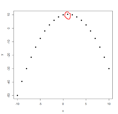
I want to choose the value of x that maximizes y, or I could fit a function and find the values of the parameters that maximize that function.

To put it simple I decide to fit a general linear regression model (quadratic on the variable) Y=a+bx+cx^2. I can do it with R, using the glm() funtcion. And I would get the values of a, b, c their standard errors SE(a), SE(b), SE(c), R2 and more things.

And the max would be located at x=-b/2c

My question is, How can I calculate the confidence interval for that x, the predictor? Is it just the typical formula x+-Z·S/sqrt(n)? and using some result provided by R for that S? or do I need to calculate that standard using a more complex methods, such as the square root of the sum of derivatives squared...? Or it's something completly different?

How would you do it with a simulation with x ? maybe calculate "y" for different values of x with perturbation. then choose the 95% max values of y (??) and calculate the confidence interval for the associated x's ? How would you do it?

$\endgroup$
8
  • 2
    $\begingroup$ If you want to stay frequentist you could look up the delta method which will provide a way to get standard errors for transformations of your parameters $\endgroup$
    – Dason
    Commented Jul 17, 2015 at 12:28
  • $\begingroup$ So do you think the delta method (what I called the square root of the sum of derivatives squared...) would be appropiate to calculate the predictor's confidence interval ? And what if I prefer the likelihood methodology? Do you know of any link with examples o further information? $\endgroup$
    – skan
    Commented Jul 17, 2015 at 17:32
  • $\begingroup$ R glm shows the standard errors for the coefficient estimates. Should I use them or the standard deviations instead? And I also need to know the error for the Y, How can I get it? From the residuals deviance, using the "confint" or how? $\endgroup$
    – skan
    Commented Jul 17, 2015 at 17:40
  • 1
    $\begingroup$ Your first question doesn't make any sense to me. And you would need to get the full covariance matrix for the predictors. You can't just use the standard errors of the estimates themselves because they are correlated. In R you would use the vcov function to get the covariance matrix from the model. $\endgroup$
    – Dason
    Commented Jul 17, 2015 at 17:44
  • $\begingroup$ Thanks, that was going to be related my next question, vcov solves it. The question aboout how to get the error associated to "y" still remains. If you create an answer joinning all your comments I could vote you. $\endgroup$
    – skan
    Commented Jul 17, 2015 at 17:47

1 Answer 1

3
$\begingroup$

In the comments there are good proposals, like the traditional delta method. A newer method which might be more exact, is constructing a profile likelihood confidence interval, which today is quite easy.

I will show below with an simulated example, in R. First write the linear regression (polynomial) model as $$ Y_i = a + b x_i + c x_i^2 + \epsilon_i $$ Now, assuming $c<0$ so as to have a maximum ... (If $c>0$ the same methods will give a confidence interval for the minimum), the maximum is at $$ M=-\frac{b}{2c} $$ $M$ is our interest (or focus) parameter, so reparametrize the regression model as $$ Y_i = a + b x_i\left( 1-\frac{x_i}{2M}\right) +\epsilon_i $$ This is now no longer linear in the parameters, but we can fit it as a nonlinear regression model:

a <- 1
b <- 1
c <- -1/2
x <- seq(from=-5,  to=5,  by=1/3)

set.seed(7*11*13) # My public seed
Y <- a + b*x  +  c*x^2  +  rnorm(length(x), 0, 2)

mydata <- data.frame(Y, x)

mod0 <- nls(Y ~ a  + b*x*(1-x/(2*M)), data=mydata,
            start=list(a=0, b=0.5, M=2))  

 summary(mod0)

Formula: Y ~ a + b * x * (1 - x/(2 * M))

Parameters:
  Estimate Std. Error t value Pr(>|t|)    
a   1.2778     0.6284   2.033   0.0516 .  
b   0.9671     0.1404   6.888 1.74e-07 ***
M   0.8975     0.1571   5.711 3.99e-06 ***
  ...  

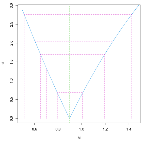
Now we call the confint function, which calls the profile function , doing likelihood profiling, and constructs the confidence interval from there:

 confint(mod0, 3)
Waiting for profiling to be done...
     2.5%     97.5% 
0.6044179 1.2658407 

We can also plot the likelihood profile for M:

Likelihood profile for parameter M

Now, as an exercise readers can compare this with the delta method ...

$\endgroup$

Your Answer

By clicking “Post Your Answer”, you agree to our terms of service and acknowledge you have read our privacy policy.

Not the answer you're looking for? Browse other questions tagged or ask your own question.