Unit root near unit circle or near 1?

Question

According to slide 6 of Bartlett's Introduction to Time Series Analysis, Lecture 6 (with emphasis on slide 6), an autoregressive time series model is stationary if the autoregressive polynomial has a root that is not on the unit circle. However, Wikipedia defines a unit root as a root having a value 1, which is a lot more specific than being on the unit circle. Which of the two is a more appropriate definition of a unit root for time series?

P.S.: I'm not sure how much this illuminates the question of whether the theory for unit root applies to roots with a magnitude of 1 or roots of real value 1.0, but if we adopt the vernacular of signal processing, then roots on the unit circle indicate marginal "stability". Any finite-time input into such a system creates a persistent output (it doesn't die, but neither does it grow geometrically). This is entirely consistent with the non-mean-reverting character of unit root time series processes. However, the latter seem to focus on step response to an impulse input, whereas marginal stability in general (where roots are not specifically real value 1.0) could yield oscillatory response. Perhaps the reason why they are not given attention in time series is because such behaviour is not typical in models for econometrics, health, and the environment. (Personally, I think it may show up in cyclical predatory/prey relationships).

In any case, I think I should my speculation immediately above as ground truth until I encounter indications to the contrary. This means that all the tests for unit roots, and all the literature on the implications of unit roots for the real world (which I admit to being unfamiliar with at present) focus on roots with real value 1.0. However, this is OK, as these are the only roots of interest for the application areas that time series are used for. This would mean that neither Wikipedia nor Barlett are wrong.

P.P.S. My comment about unit step response to shocks might be overly narrow. It only applies to random walks. Furthermore, my comment about step or oscillatory response is likely too narrow as well. I was leveraging my intuition for second order systems only, but the transfer function for a time series model is in no way restricted to 2nd order systems. Cochrane shows on page 113 (Figure 10.2) various other possibilities. In fact, on page 41, in the paragraph just preceding Section 6.2, he says that unit roots (with random walk being a single-order unit root) are just one form of non-stationarity. It's possible that the other responses in Figure 10.2 are due to roots on the unit circle at locations other than 1.0.

For the grey beards: Should this be the answer? I'm putting this out there because I'm not entirely sure.

Answer 1

Unit root in time series refers to the complex unit root on the unit circle. However in practice, or dealing with observable time series, the proceses with complex unit roots are rarely observed, whereas the unit root 1 is observed a lot. For unit root 1 implies that that the first difference of the series is stationary. First difference of a log series is simply a growth, and in economics there are lots of series with stationary growth. The most prominent example is the GDP.

The unit root processes arise a special case of ARMA processes. The ARMA process is a stationary process (covariance stationary) which satisfies the equation:

$$\phi(L)X_t= \theta(L)Z_t,$$

where $Z_t$ is a white noise process, $\phi(L)$ and $\theta(L)$ are polynomial lag operators, i.e. polynomials where $\sum_{i=0}^p\phi_iL^i$ and $\sum_{i=0}\theta_iL^i$, where $\phi_i$ and $\theta_i$ are real numbers and $L$ is the lag operator $LX_t=X_{t-1}$ (Sometimes it is called backwards operator and letter $B$ is used).

The polynomials have real coefficients, since the observable series $X_t$ are real. However for finding the conditions when the stationary process exists complex analysis is used. Wold theorem says that every covariance stationary process is actually a linear process which can be expressed as a following series:

$$X_t=\sum_{j}\psi_jZ_{t-j},$$

where $Z_t$ is a white noise process and $\sum_j|\psi_j|<\infty$. Note that this expression can be rewritten as $\sum_j\psi_jL^j$, i.e. as Laurent series. It is then natural to seek such solution for ARMA process, where we can write

$$X_t=\frac{\theta(L)}{\phi(L)}Z_t=\psi(L)Z_t,$$

with $\psi(L)=\sum_j\psi_jL^j$. To make this operational we need to make sure that $\psi(L)$ is well defined and that $\sum_j|\psi_j|<\infty$. For that we use complex analysis which says that analytic function can be expressed as a Laurent series. Since we need $\sum_j|\psi_j|<\infty$, we need that $\psi(z)$ is analytic on unit circle. Since we define $\psi(z)$ as a fraction of two analytic functions, we need that denominator is not zero on the unit circle.

And so we come to unit root process. If $\phi(z)$ has a unit root, then it can be written as either $(1-z)\phi_1(z)$, $(1+z)\phi_1(z)$ or $(1-2zcos\theta+z^2)\phi_1(z)$, where $\phi_1(z)$ is a polynomial without the unit root. The last case for the complex unit root case, where only conjugate unit roots can exist, since the coefficients of polynomial are real.

In all of these cases $\tilde Z_{t}=\frac{\theta(L)}{\phi_1(L)}Z_t$ is a stationary process we can simplify ARMA equation to the following three cases:

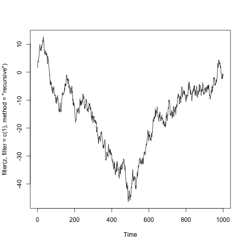
1. $X_t = X_{t-1}+ \tilde Z_t$, which corresponds to root 1,

2. $X_t = -X_{t-1}+ \tilde Z_{t}$, which corresponds to the root -1,

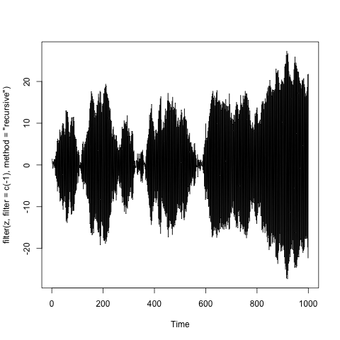
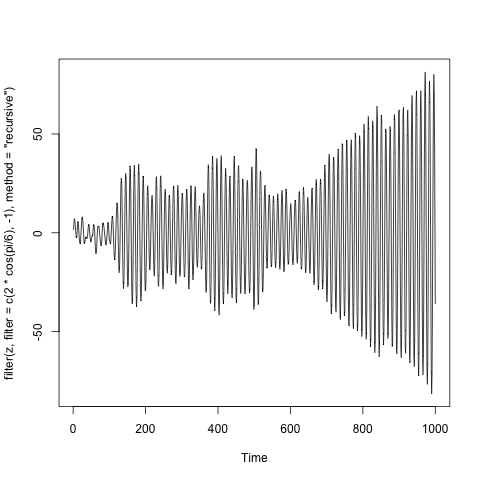
3. $X_t = 2\cos\theta X_{t-1}-X_{t-2}+\tilde Z_t$, which corresponds to conjugate complex unit root $\cos\theta\pm i\sin\theta$.

Looking at possible cases of unit root processes it is clear why the root 1 is preferred.

Below are the examples of such processes, where $\tilde Z_t$ is the a sample of one thousand independent standard normal variables. (The code is in the title of y-axis).

Note. I took some liberties with mathematics, but the general idea can be presented rigorously. The best example is the Time series lecture notes by A. van der Vaart.

Answer 2

I'm no expert in the notion of stability but I think Bartlett means all roots outside the unit circle and wikipedia is just incorrectly stated.

Note though that you need to be careful how you define the polynomial. Take for example, the AR(2). $ y_t = \phi_1 y_{t-1} + \phi_2 y_{t-2} + e_t $.

Then the AR(2) polynomial can be defined as $ (\lambda^2 - \phi_1 \lambda - \phi_2) $ or as $ (1 - \phi_1 z - \phi_2 z^2)$.

These two polynomials have roots that are reriprocals of each other. In the first case, the AR(2) is stable if the roots are inside the unit circle. In the second case, the AR(2) is stable if the roots are outside the unit circle. So be careful how you define the polynomial before deciding on the statement. For me. its more natural to define it with the z's.

All of this is in Hamilton's text which I highly recommend.