How to create a data partition in R using categorical and numerical columns? [closed]

Question

I'm using the createDataPartition method of the caret package as following:

partitionIndex = createDataPartition(paste(data$CategoricalVar1,
                                           data$CategoricalVar2,
                                           data$CategoricalVar3),
                                     p = 0.75,
                                     list = FALSE)

It works well keeping the relative proportions of the 3 categorical variables, but now I need to also consider 2 numerical variables. If I was downsampling, I would use:

predictors = c("CategoricalVar1", "CategoricalVar2", "CategoricalVar3", "NumericalVar1", "NumericalVar2")
output = c("Class")
downsampled = downSample(data[,predictors], data[,output])

And it would keep the relative proportions of all predictors. Is it possible to do the same with createDataPartition? If not, how?

Answer 1

While reading the downSample code, I realized that it doesn't keep the proportions of all predictors variables, but simply do a random stratified sampling (which is exactly what its documentation says). Inspired by downSample and createDataPartition, I wrote a createGroups function that, given a data.frame, goes through all of its columns and, if they're numeric, create quantile groups, if they're not, simply use their values, appending everything to a single list. In the end, the list should contain things like:

"[-3.54,-0.634](0.724,3.06]Class2"
"(0.715,2.86](0.724,3.06]Class1"
"(-0.634,-0.0055][-3.21,-0.677]Class1"
...

This list could then be used with createDataPartition to create the partitions. The code for that function is:

createGroups <- function (data, numericGroups = 5) {
  result <- NULL
  for (column in colnames(data)) {
    tmp <- data[,column]
    if (is.numeric(tmp)) {
      tmp <- cut(tmp,
                 unique(quantile(tmp, probs = seq(0, 1, length = numericGroups))),
                 include.lowest = TRUE)
    }

    if (is.null(result)) {
      result <- tmp
    } else {
      result <- paste0(result, tmp)
    }
  }
  result
}

On a single variable, it should be equivalent to using createDataPartition. I tested it against random sample and createDataPartition by splitting the dataset in two groups and using the Welch Two Sample t-test to test if both have equal means. The p-values should be near 1 if they do. I did 2.000 repetitions using random sampling, my createGroups function, and createDataPartition. My expectation is that my function gives results similar to createDataPartition.

The test code is:

library(caret)
library(doParallel)
library(ggplot2)

set.seed(1)
p = 0.5
data = twoClassSim(1000)[,c("Linear01", "Linear02", "Class")]

randomTest = unlist(foreach(i = 1:2000) %do% {
  set.seed(i)
  index = sample(1:nrow(data), floor(p * nrow(data)))
  t.test(data[index,]$Linear01, data[-index,]$Linear01)$p.value  
})

groups = createGroups(data)
createGroupsTest = unlist(foreach(i = 1:2000) %do% {
  set.seed(i)
  index = createDataPartition(groups, p = p)$Resample1
  t.test(data[index,]$Linear01, data[-index,]$Linear01)$p.value
})

createDataPartitionTest = unlist(foreach(i = 1:2000) %do% {
  set.seed(i)
  index = createDataPartition(data$Linear01, p = p)$Resample1
  t.test(data[index,]$Linear01, data[-index,]$Linear01)$p.value  
})

results = data.frame(p.value = c(randomTest, createGroupsTest, createDataPartitionTest),
                     class = c(rep("random", length(randomTest)),
                               rep("createGroups", length(createGroupsTest)),
                               rep("createDataPartition", length(createDataPartitionTest))))
ggplot(results, aes(x = results$p.value)) +
  theme_bw() +
  geom_density(aes(fill = class), alpha = 0.5)

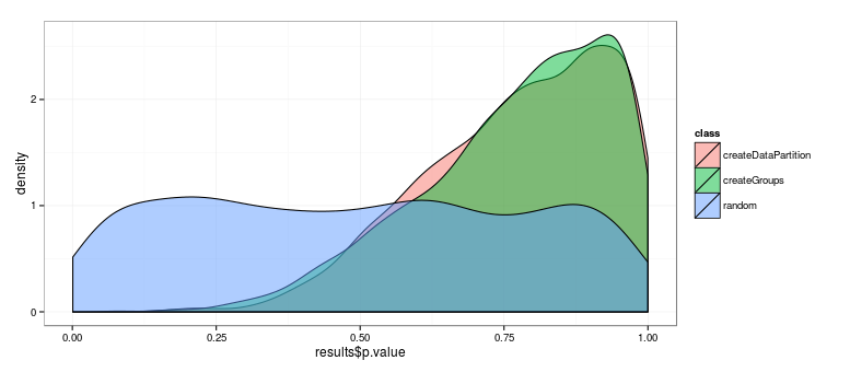
Which gives the chart:

As expected, createDataPartition and createGroups have quite similar values, with p-value of the same Welch test between the two being 0.7937281 (t.test(createGroupsTest, createDataPartitionTest)$p.value), while random sampling is quite different (p-value << 0.001, t.test(createDataPartitionTest, randomTest)$p.value), with results roughly uniform across [0, 1].

This doesn't guarantee that createGroups is correct when using multiple groups, but gives me confidence in using it.