Use ACF and PACF for irregular time series?

Question

Given an irregular daily time series where some days are missing, e.g. holidays and weekends.

Suppose data is a zoo object in R, there are two ways to plot ACF of data (PACF in the same ways):

1. acf(coredata(data))
2. acf(data, na.action = na.pass)

The first approach will reindex the data so the data will be shift to eliminate the holidays and weekend. A regular ts is thus used in ACF.

The second approach will interpolate NA in the ts. But I do not know how acf function deals with NA when na.action=na.pass is specified.

The resulting plots were quite different so which approach is the correct one?

Answer 1

The latter approach is preferred since the time difference must be invariant/constant for an ACF/PACF to be useful for model identification purposes. Intervention Detection can be iteratively used to estimate the missing values while accounting for the auto-correlative structure. One can invert the time series--i.e., go from latest to earliest to estimate missing values--and then reverse the process (normal view) to tune the missing value estimates.

Answer 2

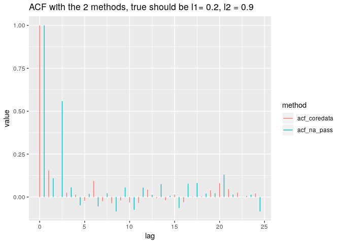
Yes, you should definitely use the second approach: if you do the first, you are considering distant observations as close. If auto-correlation is decreasing with the lag (as is usually the case) then this would lead to an under-estimation of the ACF values: indeed, using say lag 5 (low correlation) for estimating lag 1 (higher correlation) biases your results. See the plot below to see this result.

Also, no need to fill-in manually NA, as acf() is calling as.ts(), and as.ts() on a zoo object returns a vector with NA already.

library(zoo)
#> 
#> Attaching package: 'zoo'
#> The following objects are masked from 'package:base':
#> 
#>     as.Date, as.Date.numeric

N <-  5000
x <- arima.sim(model = list(ma = c(0.2, 0.9)), n = N)

set.seed(123)
index_x <-  sort(sample(1:N, size = N/5, replace = FALSE))
x_miss <-  x[index_x]

x_miss_zoo <- zoo(x_miss, order.by = index_x)


## coredata
ac_1 <- acf(coredata(x_miss_zoo), lag.max = 24, plot = FALSE)
ac_2 <- acf(x_miss_zoo,  na.action = na.pass, lag.max = 24, plot = FALSE)


library(tidyverse)
data_frame(lag = 0:24, 
           acf_coredata = ac_1$acf[,1,],
       acf_na_pass = ac_2$acf[,1,]) %>% 
  gather(method, value, -lag) %>% 
  mutate(lag = ifelse(method =="acf_coredata", lag, lag +0.5)) %>%  #kind of a hack...
  ggplot(aes(x = lag, y= value, colour = method)) +
  geom_segment(aes(xend = lag, yend = 0)) +
  ggtitle("ACF with the 2 methods, true should be l1= 0.2, l2 = 0.9")

^{Created on 2018-11-16 by the reprex package (v0.2.1)}