Relation between overfitting and Bias-variance tradeoff

Question

Consider a regression problem with training set of 5 data points being fitted with a polynomial. Its clear to me that bias is less on overfitting (use of high order polynomial) but how is variance higher than underfitting? The error decomposition is given as

Here the variance is that in the estimated model at a point , but after estimating the model, the predicted value at a particular data point is fixed and variance thus is zero for both overfitting and underfitting. So how is the variance high for overfitting than underfitting

As mentioned in Wikipedia article of Bias-variance trade-off, In error decomposition, the variance is error from sensitivity to small fluctuations in the training set. High variance can cause overfitting:

Answer 1

The decomposition that you show should be referred to the test MSE = Expected Prediction Error.

... the predicted value at a particular data point is fixed and variance thus is zero for both overfitting and underfitting.

No, the variance is not zero. The variance we are interested in measure the variability of estimated parameters, more complex the model is more high variance will be.

After passing the minimum of test MSE, If model complexity growth yet we have that: squared bias decrease, variance increase, test MSE increase. This situation represent overfitting. See graphs here:

and read related discussions there:

Is the idea of a bias-variance "tradeoff" a false construct?

When will $\text{Variance}=\text{Bias}^2$ hold for the optimal model?

However I suggest another reasoning for figured out the overfitting problem. We plot a graph (model complexity in horizontal axis) with both: test MSE and training MSE. Is easy to see that: initially both decrease but after passing a "key point" training MSE keep to decline but test MSE start to increase. So, after this key point (min test MSE) the model start to overfit. See the graph:

Answer 2

The predicted model itself is random as it is derived as a function of the data. When you think about what we are taking expectation over, it is the dataset $X$ which is used to derive the predicted model. There are two sources of randomness: one from $\epsilon$ where we assume from the model $y = f(x) + \epsilon$ where $f(x)$ is the fixed true regression function and $\epsilon$ is assumed noise, and one from $\hat f$ as previously mentioned from the randomness of the data.

Answer 3

@markowitz and @qwr are both correct, but let me say it a different way. The bias variance tradeoff is making a point about functions $\hat{f}$ that have been fit to completion, it doesn't know about gradient decent or newtons method. For a fixed hypothesis class these things manifest as an increase in bias, and a corresponding decrease in variance (heuristically). If we don't perform early stopping, then we're effectively allowing the bias to decrease within the hypothesis class, at the cost of an increase in variance. Increase in variance means it's more likely we pick a bad $\hat{f}$.

More in-depth

In this computation, we're assuming the underlying data comes from a distribution, ie that it changes with each draw. We want to know how far off out fit can be given that the $y$ values of each draw will be determined stochastically, even for fixed $x_i$ values.

In short, we don't care about a single fitting of $\hat{f}$, we're looking at the space of all possible fittings of $\hat{f}$ given the uncertainty in the underlying data. The variance is taken over these draws.

Now, the bias variance tradeoff is making a point about the best we could possibly do within the hypothesis class, that is

• What the theoretical best we could do given a certain amount of data?
• How likely are we to get close that theoretic best?

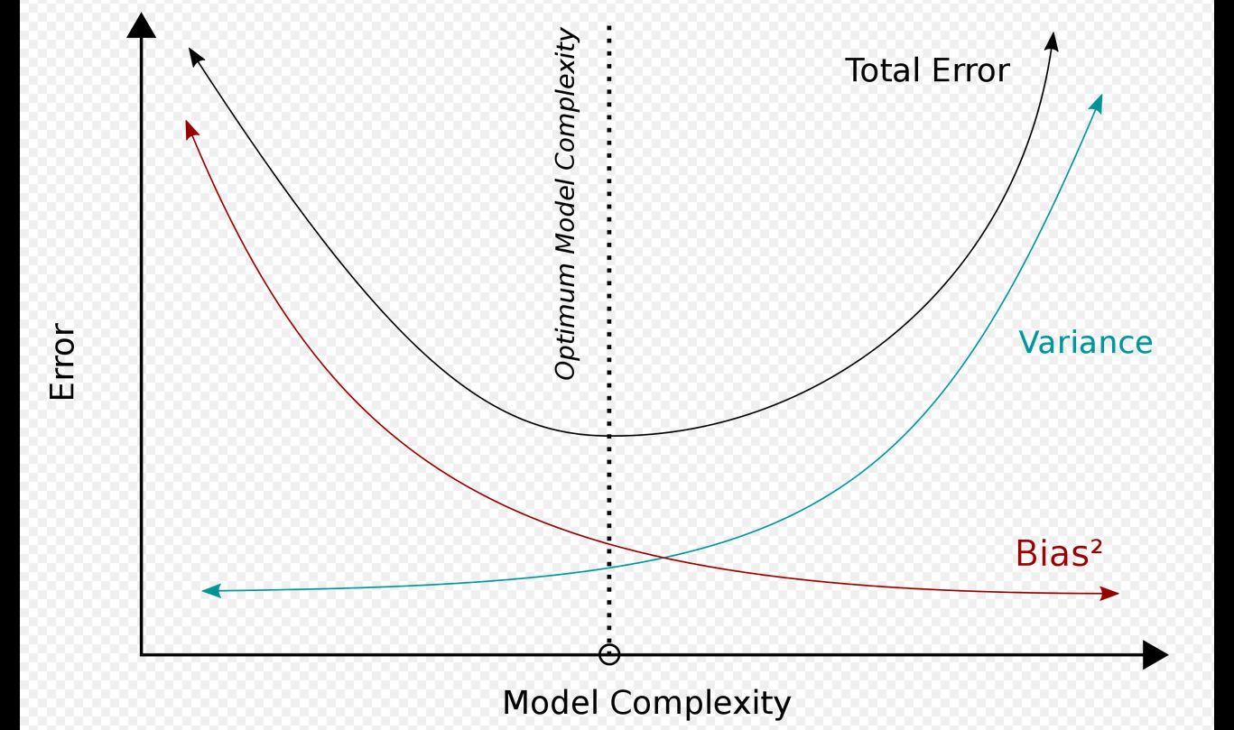
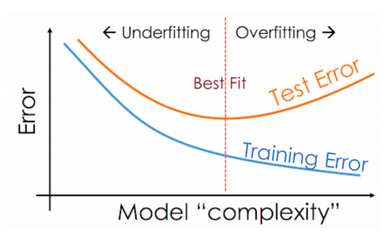
Overfitting is a consequence of the variance in the model, that is the second point. As @markowitz pointed out, given a fixed amount of data observed, the bias variance tradeoff says that as the model becomes more complex, ie as the bias lowers, the variance becomes higher. If the variance is higher, we are more likely to have picked $\hat{f}$ to be far away from the true model function $f$, even as we lower the training error.

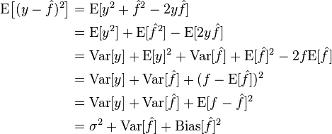
I think the screenshot of the computation above is from Elements of Statistical Learning, where they have a tendency to not say what the expectation is over. They are always assuming (as qwr pointed out) that if you draw a label $y$ from a fixed $x_0$, you don't always get the same value, there is some probability $P(y|x=x_0)$ of drawing each label.

Let $\mathcal{T} = {(x_i,yi)}$ be a training set. Then, even if the $x_i$ are fixed, the $y_i$ will be different depending on the particular sample we've taken. In the computation above the training set $\mathcal{T}$ is our independent variable, and $\hat{f} = \hat{f}(\mathcal{T})$ should be though of as a function of $\mathcal{T}$. So really, at each line of the computation we could write $$ E_{\mathcal{T}}\big[(y-\hat{f}\big] = \ldots $$ Notice that as the size of the training set $|\mathcal{T}|$ gets larger, we expect $\text{Var}_{\mathcal{T}}\big[\hat{f}\big]$ to go to 0. But for fixed $N$, we expect the variance to depend of the complexity of the function.

There's a subtlety here though, as the complexity increases the hypothesis class chances and $E_{\mathcal{T}}\big[(y-\hat{f}\big]$ also changes. It is possible that this could actually lower overall, or raise. In the case of overfitting we are often seeing a reduction in bias to close to 0, with a much larger rise in variance leading to in increase in total expected error.

Remember, the computation above assumes that fitting of $\hat{f}$ has been performed to completion, it doesn't know about gradient decent or newtons method. For a fixed hypothesis class these things manifest as an increase in bias.