I am trying to interpret my estimated paramter values with real data. In the process I made a very simple logistic regression example (GLM w/ logit link) where ground truth is available. I found that the estimated parameters were scaled versions of the ground truth parameters - furthermore the outlying probabilities (very close to 0/1) where poorly calibrated. Why is this & is there anyway to correct it?
Here is my Matlab code & example:
N = 100000; D = 10;   % N=# of observations. D=# of feautures
logit = @(x) 1./(1+exp(-x));    % defining logit/sigmoid link function
V = randn(N,D);   % randomly generated observation/design matrix from std. normal distr.
C = randn(D,1);   % randomly generated ground truth coefficients
S = logit(V*C);   % ground truth probability of firing
y = S>rand(length(N),1);   % observed binary sequence done by 'biased coin flipping'

Cp = glmfit(V,y,'binomial','link','logit','constant','off'); % Cp is est coef vector
yP = logit(V*Cp);     % esimted prob. of firing
clf;
subplot(321); plot(C,Cp);
subplot(312); I = [1:300]+1000; plot([S(I),yP(I)]);
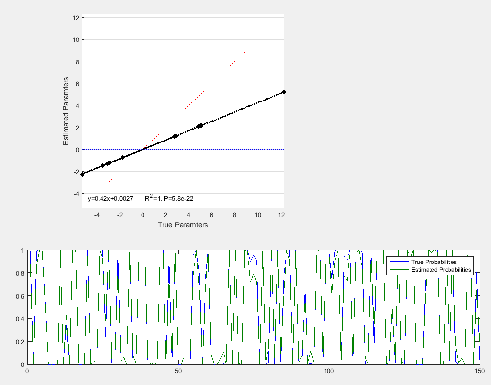
And the produced figures: Notice that in the top plot of the true vs estimated paramters, the line passes through the origin (no shift) but has a slope different than 1, as indicated by the dashed red y=x line (ie there is a scale factor). Notice in the bottom plot the outlying probabilites are slightly off.


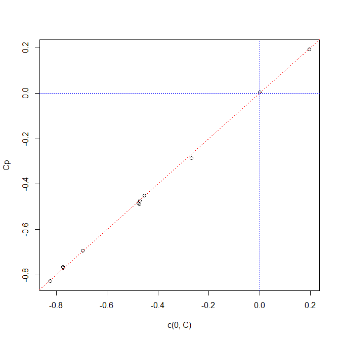
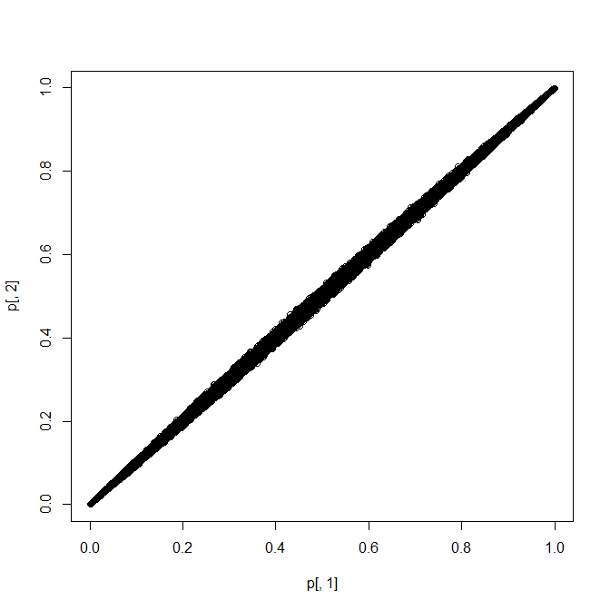
R, but my actual and estimated coefficients lay along the $y=x$ line, as expected. $\endgroup$C = randn(D,1)is generating 10 data from a standard normal, why do you have a value >12? $\endgroup$