7
$\begingroup$

I run a weighted-least squares regression to account for the heteroscedasticity in my data. When I examine the Pearson correlations between all predictor variables, I can't detect high collinearity. However, when I apply WLS with the inverse of the variance as my weights and then screen the variance inflation factors of the regression, I find VIFs far above 10.

My question is: Does WLS always suffer from multicollinearity in my case as the weighting with the inverse of the variance necessarily leads to higher dependencies of the predictors?

$\endgroup$
4
  • 1
    $\begingroup$ Just to clarify: why should weighing with the inverse of squared residuals generate dependence among the regressors? The off-diagonal elements are all still 0. Also, is there any good reason you are using WLS as opposed to OLS with robust standard errors? $\endgroup$
    – ChinG
    Commented Oct 30, 2015 at 19:10
  • 2
    $\begingroup$ How many variables do you have? What are the VIFs if you fit an OLS model ignoring the heteroscedasticity? $\endgroup$ Commented Oct 30, 2015 at 20:15
  • $\begingroup$ @ChinG Off-diagonal elements of what? Dependence among the regressors would naturally be evaluated by means of their covariance matrix (or, in the case of WLS, their weighted covariance matrix). The only times those off-diagonal elements are zero is when all regressors are orthogonal (which is rare except for designed experiments with no missing values). $\endgroup$
    – whuber
    Commented Oct 30, 2015 at 20:27
  • $\begingroup$ Off diagonal elements of the variance-covariance matrix. For WLS, we set the off diagonal elements to 0. If one wants dependence (autocorrelation, clustering etc) across error terms, one could implement a more general GLS estimator. $\endgroup$
    – ChinG
    Commented Nov 1, 2015 at 14:17

1 Answer 1

4
$\begingroup$

It's a great question, because it concerns an important and fundamental issue about multiple regression. The answer is that weighting can change the VIF (a measure of collinearity among the regressors) by arbitrary amounts up or down (with a lower limit of $1$).

To see why that is, consider a model with two regressors $X_1$ and $X_2$. (We do not have to consider the response variable: it plays no role in computing the VIF.) Here is a scatterplot of 50 observations, with the symbol areas proportional to the weights:
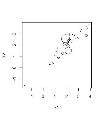
Figure

If those weights were not applied, clearly the correlation would be strongly positive, because the points line up closely along a positively sloping line. Indeed, their (unweighted) VIF is $13.54$: large enough to drive one to investigate this model carefully for effects of collinearity. (Rules of thumb assert that VIFs above $5$ or $10$ begin to be of concern.)

The weights, though, throw the correlation in altogether a different direction. The points with the heaviest weights tend to be negatively correlated: some towards the upper left, others toward the lower right. These cause the weighted correlation to be nearly zero. Indeed, the VIF for these weighted data is merely $1.44$: low and benign.

The procedure works in reverse: we could weight the data to perform an OLS and then unweight them in a WLS. Thus it's just as possible that the weighted fit will reduce the VIF as increase it.

$\endgroup$

Your Answer

By clicking “Post Your Answer”, you agree to our terms of service and acknowledge you have read our privacy policy.

Not the answer you're looking for? Browse other questions tagged or ask your own question.