How to smooth data and force monotonicity

Question

I have some data which I would like to smooth so that the smoothed points are monotonically decreasing. My data sharply decreases and then begins to plateau. Here's an example using R

df <- data.frame(x=1:10, y=c(100,41,22,10,6,7,2,1,3,1))
ggplot(df, aes(x=x, y=y))+geom_line()

What's a good smoothing technique I could use? Also, it'd be nice if I can force the 1st smoothed point to be close to my observed point.

Answer 1

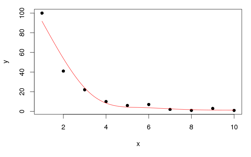
You can do this using penalised splines with monotonicity constraints via the mono.con() and pcls() functions in the mgcv package. There's a little fiddling about to do because these functions aren't as user friendly as gam(), but the steps are shown below, based mostly on the example from ?pcls, modified to suit the sample data you gave:

df <- data.frame(x=1:10, y=c(100,41,22,10,6,7,2,1,3,1))

## Set up the size of the basis functions/number of knots
k <- 5
## This fits the unconstrained model but gets us smoothness parameters that
## that we will need later
unc <- gam(y ~ s(x, k = k, bs = "cr"), data = df)

## This creates the cubic spline basis functions of `x`
## It returns an object containing the penalty matrix for the spline
## among other things; see ?smooth.construct for description of each
## element in the returned object
sm <- smoothCon(s(x, k = k, bs = "cr"), df, knots = NULL)[[1]]

## This gets the constraint matrix and constraint vector that imposes
## linear constraints to enforce montonicity on a cubic regression spline
## the key thing you need to change is `up`.
## `up = TRUE` == increasing function
## `up = FALSE` == decreasing function (as per your example)
## `xp` is a vector of knot locations that we get back from smoothCon
F <- mono.con(sm$xp, up = FALSE)   # get constraints: up = FALSE == Decreasing constraint!

Now we need to fill in the object that gets passed to pcls() containing details of the penalised constrained model we want to fit

## Fill in G, the object pcsl needs to fit; this is just what `pcls` says it needs:
## X is the model matrix (of the basis functions)
## C is the identifiability constraints - no constraints needed here
##   for the single smooth
## sp are the smoothness parameters from the unconstrained GAM
## p/xp are the knot locations again, but negated for a decreasing function
## y is the response data
## w are weights and this is fancy code for a vector of 1s of length(y)
G <- list(X = sm$X, C = matrix(0,0,0), sp = unc$sp,
          p = -sm$xp, # note the - here! This is for decreasing fits!
      y = df$y,
          w = df$y*0+1)
G$Ain <- F$A    # the monotonicity constraint matrix
G$bin <- F$b    # the monotonicity constraint vector, both from mono.con
G$S <- sm$S     # the penalty matrix for the cubic spline
G$off <- 0      # location of offsets in the penalty matrix

Now we can finally do the fitting

## Do the constrained fit 
p <- pcls(G)  # fit spline (using s.p. from unconstrained fit)

p contains a vector of coefficients for the basis functions corresponding to the spline. To visualize the fitted spline, we can predict from the model at 100 locations over the range of x. We do 100 values so as to get a nice smooth line on the plot.

## predict at 100 locations over range of x - get a smooth line on the plot
newx <- with(df, data.frame(x = seq(min(x), max(x), length = 100)))

To generate predicted values we use Predict.matrix(), which generates a matrix such that when multiple by coefficients p yields predicted values from the fitted model:

fv <- Predict.matrix(sm, newx) %*% p
newx <- transform(newx, yhat = fv[,1])

plot(y ~ x, data = df, pch = 16)
lines(yhat ~ x, data = newx, col = "red")

This produces:

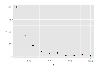
I'll leave it up to you to get the data into a tidy form for plotting with ggplot...

You can force a closer fit (to partially answer your question about having the smoother fit the first data point) by increasing the dimension of the basis function of x. For example, setting k equal to 8 (k <- 8) and rerunning the code above we get

You can't push k much higher for these data, and you have to be careful about over fitting; all pcls() is doing is solving the penalised least squares problem given the constraints and the supplied basis functions, it's not performing smoothness selection for you - not that I know of...)

If you want interpolation, then see the base R function ?splinefun which has Hermite splines and cubic splines with monotonicty constraints. In this case you can't use this however as the data are not strictly monotonic.

Answer 2

The recent scam package by Natalya Pya and based on the paper "Shape constrained additive models" by Pya & Wood (2015) can make part of the process mentioned in Gavin's excellent answer much easier.

library(scam)
con <- scam(y ~ s(x, k = k, bs = "mpd"), data = df)
plot(con)

There are a number of bs functions you can use - in the above I used mpd for "monotonic decreasing P-spline" but it also has functions that enforce convexity or concavity either separately or alongside the monotonic constraints.