How to perform non-negative ridge regression?

Question

How to perform non-negative ridge regression? Non-negative lasso is available in scikit-learn, but for ridge, I cannot enforce non-negativity of betas, and indeed, I am getting negative coefficients. Does anyone know why this is?

Also, can I implement ridge in terms of regular least squares? Moved this to another question: Can I implement ridge regression in terms of OLS regression?

Answer 1

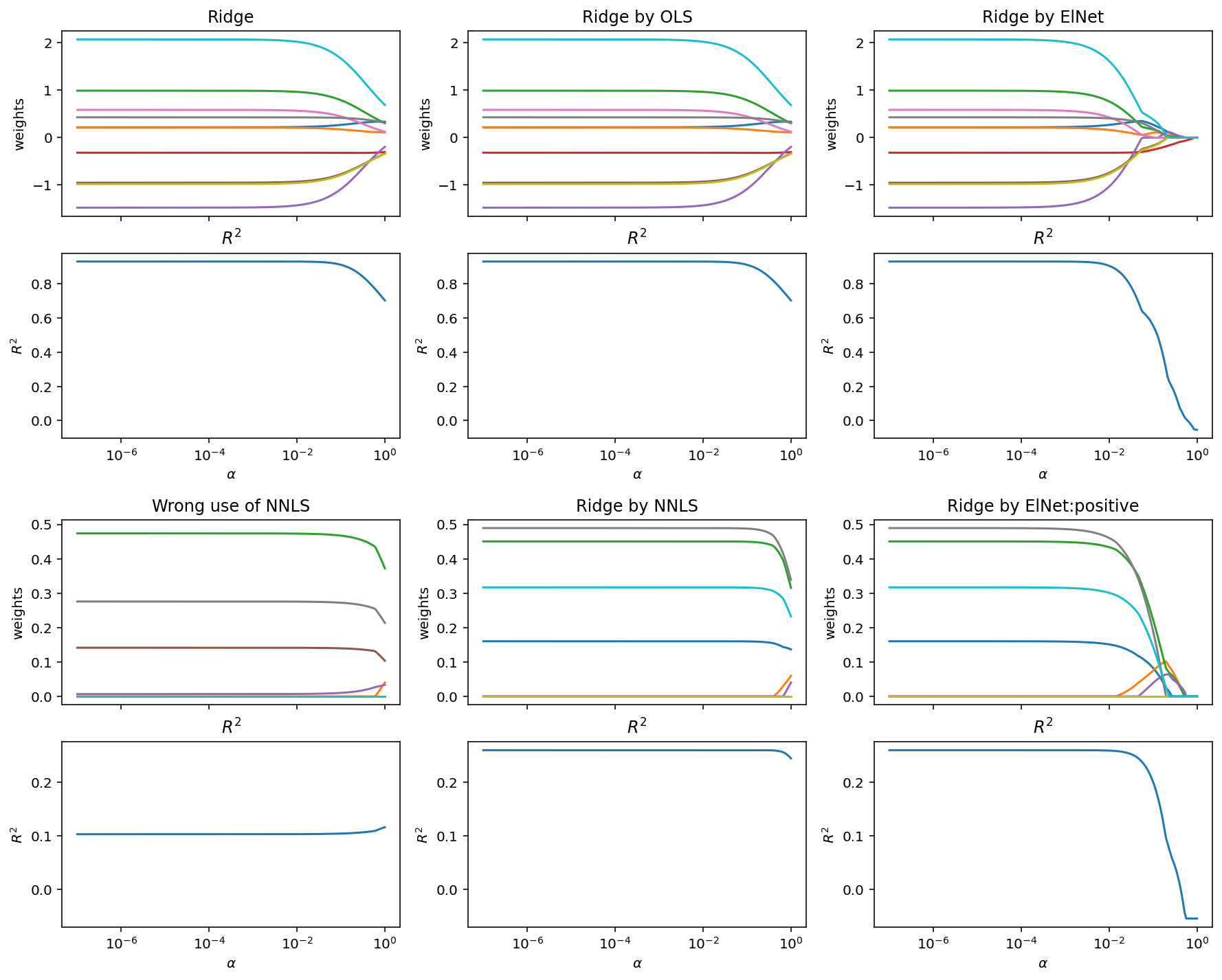
The rather anti-climatic answer to "Does anyone know why this is?" is that simply nobody cares enough to implement a non-negative ridge regression routine. One of the main reasons is that people have already started implementing non-negative elastic net routines (for example here and here). Elastic net includes ridge regression as a special case (one essentially set the LASSO part to have a zero weighting). These works are relatively new so they have not yet been incorporated in scikit-learn or a similar general use package. You might want to inquire the authors of these papers for code.

EDIT:

As @amoeba and I discussed on the comments the actual implementation of this is relative simple. Say one has the following regression problem to:

$y = 2 x_1 - x_2 + \epsilon, \qquad \epsilon \sim N(0,0.2^2)$

where $x_1$ and $x_2$ are both standard normals such as: $x_p \sim N(0,1)$. Notice I use standardised predictor variables so I do not have to normalise afterwards. For simplicity I do not include an intercept either. We can immediately solve this regression problem using standard linear regression. So in R it should be something like this:

rm(list = ls()); 
library(MASS); 
set.seed(123);
N = 1e6;
x1 = rnorm(N)
x2 = rnorm(N)
y = 2 * x1 - 1 * x2 + rnorm(N,sd = 0.2)

simpleLR = lm(y ~ -1 + x1 + x2 )
matrixX = model.matrix(simpleLR); # This is close to standardised
vectorY = y
all.equal(coef(simpleLR), qr.solve(matrixX, vectorY), tolerance = 1e-7)  # TRUE

Notice the last line. Almost all linear regression routine use the QR decomposition to estimate $\beta$. We would like to use the same for our ridge regression problem. At this point read this post by @whuber; we will be implementing exactly this procedure. In short, we will be augmenting our original design matrix $X$ with a $\sqrt{\lambda}I_p$ diagonal matrix and our response vector $y$ with $p$ zeros. In that way we will be able to re-express the original ridge regression problem $(X^TX + \lambda I)^{-1} X^Ty$ as $(\bar{X}^T\bar{X})^{-1} \bar{X}^T\bar{y}$ where the $\bar{}$ symbolises the augmented version. Check slides 18-19 from these notes too for completeness, I found them quite straightforward. So in R we would some like the following:

myLambda = 100;  
simpleRR = lm.ridge(y ~ -1 + x1 + x2, lambda = myLambda)
newVecY = c(vectorY, rep(0, 2))
newMatX = rbind(matrixX, sqrt(myLambda) * diag(2))
all.equal(coef(simpleRR), qr.solve(newMatX, newVecY), tolerance = 1e-7)  # TRUE

and it works. OK, so we got the ridge regression part. We could solve in another way though, we could formulate it as an optimisation problem where the residual sum of squares is the cost function and then optimise against it, ie. $ \displaystyle \min_{\beta} || \bar{y} - \bar{X}\beta||_2^2$. Sure enough we can do that:

myRSS <- function(X,y,b){ return( sum( (y - X%*%b)^2 ) ) }
bfgsOptim = optim(myRSS, par = c(1,1), X = newMatX, y= newVecY, 
                  method = 'L-BFGS-B')
all.equal(coef(simpleRR), bfgsOptim$par, check.attributes = FALSE, 
          tolerance = 1e-7) # TRUE

which as expected again works. So now we just want : $ \displaystyle \min_{\beta} || \bar{y} - \bar{X}\beta||_2^2$ where $\beta \geq 0$. Which is simply the same optimisation problem but constrained so that the solution are non-negative.

bfgsOptimConst = optim(myRSS, par = c(1,1), X=newMatX, y= newVecY, 
                       method = 'L-BFGS-B', lower = c(0,0))
all(bfgsOptimConst$par >=0)  # TRUE
(bfgsOptimConst$par) # 2.000504 0.000000

which shows that the original non-negative ridge regression task can be solved by reformulating as a simple constrained optimisation problem. Some caveats:

1. I used (practically) normalised predictor variables. You will need to account of the normalisation yourself.
2. Same thing goes for the non normalisation of the intercept.
3. I used optim's L-BFGS-B argument. It is the most vanilla R solver that accepts bounds. I am sure that you will find dozens of better solvers.
4. In general constraint linear least-squares problems are posed as quadratic optimisation tasks. This is an overkill for this post but keep in mind that you can get better speed if needed.
5. As mentioned in the comments you could skip the ridge-regression as augmented-linear-regression part and directly encode the ridge cost function as an optimisation problem. This would be a lot simpler and this post significantly smaller. For the sake of argument I append this second solution too.
6. I am not fully conversational in Python but essentially you can replicate this work by using NumPy's linalg.solve and SciPy's optimize functions.
7. To pick the hyperparameter $\lambda$ etc. you just do the usual CV-step you would do in any case; nothing changes.

Code for point 5:

myRidgeRSS <- function(X,y,b, lambda){ 
                return( sum( (y - X%*%b)^2 ) + lambda * sum(b^2) ) 
              }
bfgsOptimConst2 = optim(myRidgeRSS, par = c(1,1), X = matrixX, y = vectorY,
                        method = 'L-BFGS-B', lower = c(0,0), lambda = myLambda)
all(bfgsOptimConst2$par >0) # TRUE
(bfgsOptimConst2$par) # 2.000504 0.000000

Answer 2

R package glmnet that implements elastic net and therefore lasso and ridge allows this. With parameters lower.limits and upper.limits, you can set a minimum or a maximum value for each weight separately, so if you set lower limits to 0, it will perform nonnegative elastic-net (lasso/ridge).

There is also a python wrapper https://pypi.python.org/pypi/glmnet/2.0.0

Answer 3

I know it's an oldie, but I put an example here of how to do this in Python either by using ElasticNet (approximation), or via nnls().

Basically, for ElasticNet, you can use:

from sklearn import linear_model as lm

eln = lm.ElasticNet(l1_ratio=0, fit_intercept=False)
act_alphas, coefs, dual_gaps = eln.path(X, y, alphas=alphas, positive=True)

but be forewarned that ElasticNet spews a lot of warnings for large values of alpha, as it doesn't converge.

Via nnls():

from scipy.optimize import nnls

def nnls_ridge(X, y, alpha):
    """return non-negative Ridge coefficients"""
    p = X.shape[1]
    Xext = np.vstack((X, alpha * np.eye(p)))
    yext = np.hstack((y, np.zeros(p)))
    coefs, _ = nnls(Xext, yext)
    return coefs

Note

(Following the notations of this excellent post).

While it is true that in an unconstrained setting, the OLS formulation of Ridge:

$$(X_{*}^\prime X_{*})\beta = X_{*}^\prime y_{*}.$$

is equivalent to:

$$(X^\prime X + \lambda I)\beta = X^\prime y.$$

in a constrained setting (e.g. bounds = (0, np.inf), or using nnls()), the two are not equivalent, as $(X^\prime X + \lambda I)$ has already been reduced to a $p \times p$ matrix by (unconstrained) LS projection.

In particular, my initial attempt at nnls_ridge() is wrong:

def nnls_ridge_wrong(X, y, alpha):
    p = X.shape[1]
    Xmod = X.T @ X + alpha * np.eye(p)
    ymod = X.T @ y
    coefs, _ = nnls(Xmod, ymod)
    return coefs

Example (using the functions described in the GitHub link at the beginning of this post):

X = np.arange(6).reshape((-1, 2))
y = np.array([8,1,1])
a = 0.001

>>> ols_ridge(X, y, a)
array([-8.56345838,  6.81837427])

>>> nn_ridge_path_via_elasticnet(X, y, [a])[1].T
array([[0.        , 0.45708041]])

>>> nnls_ridge(X, y, a)
array([0.        , 0.45714284])

>>> nnls_ridge_wrong(X, y, a)
array([0.        , 0.37663842])

For a $X_{12,10}$ and $y_{12}$ where all components are Normal $N(0,1)$, we see some drastic differences of $R^2$ for the nnls_ridge_wrong (bottom left pair of plots):

Answer 4

Recall we are trying to solve:

$$ \text{minimize}_{x}\,\,\,\,\left\Vert Ax-y\right\Vert _{2}^{2}+ \lambda \| x \|^2_2 \,\,\,\,\text{s.t. }x>0 $$

is equivalent to:

$$ \text{minimize}_{x}\,\,\,\,\left\Vert Ax-y\right\Vert _{2}^{2}+ \lambda x^\top I x \,\,\,\,\text{s.t. }x>0 $$

with some more algebra:

$$\text{minimize}_{x}\,\,\,\,x^{T}\left(A^{T}A+ \lambda I \right)x+\left(-2A^{T}y\right)^{T}x\,\,\,\,\text{s.t. }x>0$$

The solution in pseudo-python is simply to do:

Q = A'A + lambda*I
c = - A'y
x,_ = scipy.optimize.nnls(Q,c)

---

see: How does one do sparse non-negative least squares using $K$ regularizers of the form $x^\top R_k x$?

for a slightly more general answer.