Let $x_t$ be the sequence of sensor values at each time period. We can model your approximate derivative (a.k.a. secant) as:
$$\bar {x'}_t = \frac{x_{t+1}-x_t}{\Delta t}$$
Where I am using the fact that, for continuous functions, the secant is equal to the average value of the derivative over that interval. Also, these are "forward derivatives", since the derivative at time $t$ is defined by looking at $t+1$.
Since $\Delta t$ is constant, this makes things much simpler, since only the numerator is random. To get a variance, we apply the well-known variance formula for the sum (or difference) of two iid random variables:
$$\sigma^2_{\bar{x'}} = \frac{1}{(\Delta t)^2}(\sigma^2_{x_{t+1}}+\sigma^2_{x_{t}}) = \frac{2\sigma^2_x}{(\Delta t)^2} $$
The middle step assumed that the variables were independent, the last step assumed they were identically distributed as well. This may be a very bad set of assumptions, depending on the process you are monitoring. So, let's just go with the full version, and assume that they are not independent but they are identically distributed:
$$\sigma^2_{\bar{x'}} = 2\frac{\sigma^2_{x_t}-\sigma^2_{x_t,x_{t+1}}}{(\Delta t)^2}$$
Where $\sigma^2_{x_t,x_{t+1}}$ is the covariance between the two sensor readings. It is subtracted because we preserve signs in covariances but it also makes sense intuitively: if two terms in a difference increase or decrease by a similar amount (and direction) then the difference will not change much.
We can estimate this variance using sample statistics:
Sample variance: $\widehat {\sigma^2_x} = \frac{\sum (x_t - \bar x)^2}{n-1}$
Sample covariance $\widehat {\sigma^2_{x_t,x_{t+1}}}=\frac{\sum_{i=1}^{n-1}(x_{i+1}-\bar x)(x_i-\bar x)}{n-1}$
Using the above you will be able to estimate the variance of the secant line of the measured quantity.
What about $y$?
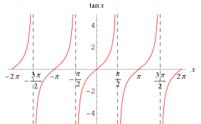
This is tricky because $tan(\theta)$ looks like this:

Which is problematic due to the discontinuities. Even assuming that $0\deg \leq \theta \leq 90 \deg$, you can see that the derivative becomes very large near the discontinuities. Therefore, the variance of the derivative of $y$ will become highly erratic near the endpoints. You will need to know how accurately you can measure $\theta$ and if the value approaches the endpoints.
Variance of y
The OP has indicated that $\theta \in (-30 \deg,30 \deg) = (-\pi/6 \;\mathrm{rad} ,\pi/6 \;\mathrm{rad})$, which is a nice range for the $tan$ curve. In fact, the slope only varies from 1 to 1.33! So, it is well approximated by a line with slope $\approx 1.2$ (the average value of the slope over the range of $\theta$) and intercept $0$.
So, we can get a good approximation of $y$ with much less analytical overhead if we use:
$$y\approx 1.2\theta x\;\; \mathrm{where}\;\; \theta\;\; \mathrm{ in \;radians}$$
Now, we can approximate the variance of $y$:
$$\sigma^2_y \approx 1.2^2\sigma^2_{\theta x}$$
So...what is $\sigma^2_{\theta x}$?! It depends on if we think $\theta$ and $x$ are independent or correlated...I'm assuming the more general case of them being correlated:
$$Var(\theta x) = E[\theta^2x^2] - (E[\theta x])^2$$
Let's rewrite using covariance:
$$Var(\theta x) = E[\theta^2x^2] - (Cov(\theta x)+ \mu_x\mu_{\theta})^2$$
We can use sample estimators of each of these terms to estimate $Var(\theta x)$:
$$\widehat{E[\theta^2x^2]} = \frac{\sum_{i=1}^n (\theta_ix_i)^2}{n}$$
$$\widehat{\mu_x} = \frac{\sum_{i=1}^n x_i}{n}$$
and you know how to calculate $cov$ from the earlier equation.
Once you have $\widehat{\sigma^2_{\theta x}}$, just multiply by $1.2^2$ to get $\widehat{\sigma^2_{y}}$

