5
$\begingroup$

I have a bivariate normal distribution composed of the univariate normal distributions $X_1$ and $X_2$ with $\rho \approx 0.3$.

$$ \begin{pmatrix} X_1 \\ X_2 \end{pmatrix} \sim \mathcal{N} \left( \begin{pmatrix} \mu_1 \\ \mu_2 \end{pmatrix} , \begin{pmatrix} \sigma^2_1 & \rho \sigma_1 \sigma_2 \\ \rho \sigma_1 \sigma_2 & \sigma^2_2 \end{pmatrix} \right) $$

Is there a simple way to calculate in R the cumulative probability of $X_1$ being less than a value $z$ given a particular slice of $X_2$ (between two values $a,b$) given we know all the parameters $\mu_1, \mu_2, \sigma_1, \sigma_2, \rho$?

$P(X_1 < z | a < X_2 < b)$

Can the distribution function I am looking for match (or be approximated by) the distribution function of a univariate normal distribution (to use qnorm/pnorm)? Ideally this would be the case so I can perform the calculation with less dependencies on libraries (e.g. on a MySQL server).

This is the bivariate distribution I am using:

means <- c(79.55920, 52.29355)
variances <- c(268.8986, 770.0212)
rho <- 0.2821711

covariancePartOfMatrix <- sqrt(variances[1]) * sqrt(variances[2]) * rho
sigmaMatrix <- matrix(c(variances[1],covariancePartOfMatrix,covariancePartOfMatrix,variances[2]), byrow=T, ncol=2)

n <- 10000
dat <- MASS::mvrnorm(n=n, mu=means, Sigma=sigmaMatrix)

plot(dat)

This is my numerical attempt to get the correct result. However it uses generated data from the bivariate distribution and I'm not convinced it will give the correct result.

a <- 79.5
b <- 80.5
z <- 50

sliceOfDat <- subset(data.frame(dat), X1 > a, X1 < b)
estimatedMean <- mean(sliceOfDat[,c(2)])
estimatedDev <- sd(sliceOfDat[,c(2)])

estimatedPercentile <- pnorm(z, estimatedMean, estimatedDev)

Edit - R implementation of solution based on whuber's answer

Here is an implementation of the accepted solution using integrate, compared against my original idea based on sampling. The accepted solution provides the expected output 0.5, whereas my original idea deviated by a significant amount (0.41). Update - See wheber's edit for a better implementation.

# Bivariate distribution parameters
means <- c(79.55920, 52.29355)
variances <- c(268.8986, 770.0212)
rho <- 0.2821711

# Generate sample data for bivariate distribution
n <- 10000

covariancePartOfMatrix <- sqrt(variances[1]) * sqrt(variances[2]) * rho
sigmaMatrix <- matrix(c(variances[1],covariancePartOfMatrix,covariancePartOfMatrix,variances[2]), byrow=T, ncol=2)
dat <- MASS::mvrnorm(n=n, mu=means, Sigma=sigmaMatrix)

# Input parameters to test the estimation
w = 79.55920

a <- w - 0.5
b <- w + 0.5
z <- 52.29355

# Univariate approximation using randomness
sliceOfDat <- subset(data.frame(dat), X1 > a, X1 < b)
estimatedMean <- mean(sliceOfDat[,c(2)])
estimatedDev <- sd(sliceOfDat[,c(2)])

estimatedPercentile <- pnorm(z, estimatedMean, estimatedDev)
# OUTPUT: 0.411

# Numerical approximation from exact solution
adaptedZ <- (z - means[2]) / sqrt(variances[2])
adaptedB <- (b - means[1]) / sqrt(variances[1])
adaptedA <- (a - means[1]) / sqrt(variances[1])

exactSolutionCoeff <- 1 / (pnorm(adaptedB) - pnorm(adaptedA))
integrand <- function(x) pnorm((adaptedZ - rho * x) / sqrt(1 - rho * rho)) * dnorm(x)
exactSolutionInteg <- integrate(integrand, adaptedA, adaptedB)
# 0.0121, abs.error 1.348036e-16, "OK"
exactPercentile = exactSolutionCoeff * exactSolutionInteg$value
# OUTPUT: 0.500
$\endgroup$
0

1 Answer 1

6
$\begingroup$

Yes, a Normal approximation works--but not in all cases. We need to do some analysis to identify when the approximation is a good one.

Exact solution

Re-express $(X_1,X_2)$ in standardized units so that they have zero means and unit variances. Letting $\Phi$ be the standard Normal distribution function (its CDF), it is well known from the theory of ordinary least squares regression that

$$\Pr(X_1 \le z\,|\, X_2 = x) = \Phi\left(\frac{z - \rho x}{\sqrt{1-\rho^2}}\right).$$

The desired probability then can be obtained by integrating:

$$\eqalign{\Pr(X_1 \le z\,|\, a \lt X_2 \le b) &= \frac{1}{\Phi(b)-\Phi(a)}\int_a^b \Pr(X_1\le z\,|\, X_2=x) \phi(x)\,dx \\&= \frac{1}{\Phi(b)-\Phi(a)}\int_a^b \Phi\left(\frac{z - \rho x}{\sqrt{1-\rho^2}}\right) \phi(x)\,dx.}$$

This appears to require numerical integration (although the result for $(a,b)=\mathbb{R}$ is obtainable in closed form: see How can I calculate $\int^{\infty}_{-\infty}\Phi\left(\frac{w-a}{b}\right)\phi(w)\,\mathrm dw$).

Approximating the distribution

This expression can be differentiated under the integral sign (with respect to $z$) to obtain the PDF,

$$f(z\,|\, a \lt X_2 \le b) = \phi(z)\ \frac{\Phi\left(\frac{b-\rho z}{\sqrt{1-\rho^2}}\right) - \Phi\left(\frac{a-\rho z}{\sqrt{1-\rho^2}}\right)}{\Phi(b) - \Phi(a)}.$$

This exhibits the PDF as product of the standard Normal PDF $\phi$ and a "correction". When $b-a$ is small compared to $\sqrt{1-\rho^2}$ (specifically, when $(b-a)^2 \ll 1-\rho^2$), we might approximate the difference in the numerator with the first derivative:

$$\Phi\left(\frac{b-\rho z}{\sqrt{1-\rho^2}}\right) - \Phi\left(\frac{a-\rho z}{\sqrt{1-\rho^2}}\right)\approx \phi\left(\frac{(a+b)/2-\rho z}{\sqrt{1-\rho^2}}\right)\frac{b-a}{\sqrt{1-\rho^2}}.$$

The error in this approximation is uniformly bounded (across all values of $z$) because the second derivative of $\Phi$ is bounded.

With this approximation, and completing the square, we obtain

$$f(z\,|\, a \lt X_2 \le b) \approx \phi\left(z; \rho(a+b)/2, \sqrt{1-\rho^2}\right) \frac{(b-a)\exp\left(-(a+b)^2/8\right)}{(\Phi(b)-\Phi(a))\sqrt{2\pi}}.$$

($\phi(*; \mu, \sigma)$ denotes the PDF of a Normal distribution of mean $\mu$ and standard deviation $\sigma$.)

Moreover, the right hand factor (which does not depend on $z$) must be very close to $1$, because the $\phi$ term integrates to unity, whence

$$f(z\,|\, a \lt X_2 \le b) \approx \phi\left(z; \rho(a+b)/2, \sqrt{1-\rho^2}\right).$$

All this makes very good sense: the conditional distribution of $X_1$ is approximated by its conditional distribution at the midpoint of the interval, $(a+b)/2$, where it has mean $\rho(a+b)/2$ and standard deviation $\sqrt{1-\rho^2}$. The error is proportional to the width of the interval $b-a$ and to an expression dominated by $\exp(-(a+b)^2/8)$, which becomes important only when both $a$ and $b$ are out in the same tail. Therefore, this Normal approximation works for narrow slices not too far into the tails of the bivariate distribution. Moreover, the difference between

$$\frac{(b-a)\exp\left(-(a+b)^2/8\right)}{(\Phi(b)-\Phi(a))\sqrt{2\pi}}$$

and $1$ serves as an excellent check of the quality of the approximation.


Edit

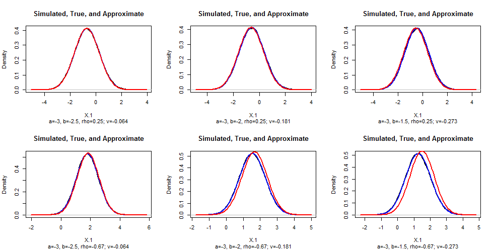
To check these conclusions, I simulated data in R for various values of $b$ and $\rho$ ($a=-3$ in all cases), drew their empirical density, and superimposed on that the theoretical (blue) and approximate (red) densities for comparison. (You cannot see the density plots because the theoretical plots fit over them almost perfectly.) As $|\rho|$ gets close to $1$, the approximation grows poorer: this deserves further study. Clear the approximation is excellent for sufficiently small values of $b-a$.

Figure

#
# Numerical integration, to give a correct value.
#
f <- function(z, a, b, rho, value.only=FALSE, ...) {
  g <- function(x) pnorm((z - rho*x)/sqrt(1-rho^2)) * dnorm(x) / (pnorm(b) - pnorm(a))
  u <- integrate(g, a, b, ...)
  if (value.only) return(u$value) else return(u)
}
#
# Set up the problem.
#
a <- -3  # Left endpoint
n <- 1e5 # Simulation size
par(mfrow=c(2,3))
for (rho in c(1/4, -2/3)) {
  for (b in c(-2.5, -2, -1.5)) {
    z <- seq((a-3)*rho, (b+3)*rho, length.out=101)
    #
    # Check the approximation (`v` needs to be small).
    #
    v <- (b-a) * exp(-(a+b)^2/8) / (pnorm(b) - pnorm(a)) / sqrt(2*pi) - 1
    #
    # Simulate some values of (x1, x2).
    #
    x.2 <- qnorm(runif(n, pnorm(a), pnorm(b)))  # Normal between `a` and `b`
    x.1 <- rho*x.2 + rnorm(n, sd=sqrt(1-rho^2))
    #
    # Compare the simulated distribution to the theoretical and approximate
    # densities.
    #
    x.hat <- density(x.1)
    plot(x.hat, type="l", lwd=2, 
         main="Simulated, True, and Approximate",
         sub=paste0("a=", round(a,2), ", b=", round(b, 2), ", rho=", round(rho, 2), 
         "; v=", round(v,3)),
         xlab="X.1", ylab="Density")

    # Theoretical
    curve(dnorm(x) * (pnorm((b-rho*x)/sqrt(1-rho^2)) - pnorm((a-rho*x)/sqrt(1-rho^2))) /
       (pnorm(b) - pnorm(a)), lwd=2, col="Blue", add=TRUE)

    # Approximate
    curve(dnorm(x, rho*(a+b)/2, sqrt(1-rho^2)), col="Red", lwd=2, add=TRUE)
  }
}
$\endgroup$
5
  • $\begingroup$ Thank you for the detailed answer. I had found that the normal approximation stopped producing the figures I expected when z was high or low. Your examination of the numerical analysis corresponds exactly to what I noticed varying a, b, and z, and makes me confident that I can get a better result by using the exact solution that you provided. $\endgroup$ Commented May 20, 2016 at 11:54
  • $\begingroup$ Would it be possible to add a little more detail on how to calculate the exact solution without numerical integration? An example line in R would be perfect. The part I am most confused about is how to convert the limits and sign of x in the integral ∫baΦ(z−ρx1−ρ2−−−−−√)ϕ(x)dx into the form ∫∞−∞Φ(w−ab)ϕ(w)dw∫−∞∞Φ(w−ab)ϕ(w)dw) so that I can use the result proved in the question that you linked. $\endgroup$ Commented May 20, 2016 at 11:58
  • 1
    $\begingroup$ Unfortunately there is no such conversion. Numerical integration really is needed. You could also pursue the development of the approximation further by using higher-order approximations to the $\Phi$ term in the integrand. Intuitively, the midpoint $(a+b)/2$ ought to be replaced by a point closer to the smaller of $a$ and $b$ (in size), because that's where most of the $X_2$ probability is. $\endgroup$
    – whuber
    Commented May 20, 2016 at 12:26
  • $\begingroup$ I've added a R example based on the exact solution -- using the mean & variance, the approximate solution was 0.41 and the exact 0.5. I am surprised how far the approximate solution is out in that case. Thanks again! $\endgroup$ Commented May 20, 2016 at 20:17
  • 1
    $\begingroup$ I saw that code, but it's not clear how it works or whether it's correct. At the very least you should compute the check value (at the end of my original post), look at $|b-a|/\sqrt{1-\rho^2}$ (in standardized units), and inspect the output of integrate to make sure it's not running into accuracy problems. $\endgroup$
    – whuber
    Commented May 20, 2016 at 20:20

Your Answer

By clicking “Post Your Answer”, you agree to our terms of service and acknowledge you have read our privacy policy.

Not the answer you're looking for? Browse other questions tagged or ask your own question.