Interpreting multinomial logistic regression in scikit-learn

Question

I am running a multinomial logistic regression for a classification problem involving 6 classes and four features.

Here is the code:

from sklearn.linear_model import LogisticRegression
from sklearn.cross_validation import train_test_split    

X_train, X_test, Y_train, Y_test = train_test_split(X, Y, test_size=0.20)

logreg = LogisticRegression(multi_class = 'multinomial', solver = 'newton-cg')
logreg = logreg.fit(X_train, Y_train)
output2 = logreg.predict(X_test)

logreg.intercept_
logreg.coef_
logreg.classes_

And I get the following output:

Intercept

array([-1.33803785, -1.55807614, -1.63809549, -0.05199907,  3.72777888, 0.85842968])

Coefficients

array([[  3.59830486,   5.1370334 ,   1.32336325,   4.89734568],
       [  3.5507364 ,   5.2459697 ,   1.48523684,   4.81653704],
       [  3.35193267,   5.40124363,   2.04869296,   3.885547  ],
       [ -5.4930705 ,   5.49483357,   1.96479926,  -6.7624365 ],
       [ -8.61513183,  -3.77761893,  -7.79363153, -11.72171457],
       [  3.6072284 , -17.50146139,   0.97153921,   4.88472135]])

Classes

array([u'Dropper', u'Flat', u'Grower', u'New User', u'Non User', u'Stopper'], dtype=object)

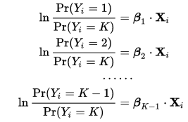
I am not able to interpret the models. As I understand multinomial logistic regression, for K possible outcomes, running K-1 independent binary logistic regression models, in which one outcome is chosen as a "pivot" and then the other K-1 outcomes are separately regressed against the pivot outcome.

As per this, there must be 5 equations for the 6 classes. But here there are 6. How come?

Answer 1

As the probabilities of each class must sum to one, we can either define n-1 independent coefficients vectors, or n coefficients vectors that are linked by the equation \sum_c p(y=c) = 1.

The two parametrization are equivalent. See also in Wikipedia Multinomial logistic regression - As a log-linear model.

For a class c, we have a probability P(y=c) = e^{b_c.X} / Z, with Z a normalization that accounts for the equation \sum_c P(y=c) = 1. These probabilities are the expected probabilities of a class given the coefficients. They can be computed with predict_proba

---

To have better insight of the coefficients, please consider the left plot in this example. example http://scikit-learn.org/dev/_images/plot_logistic_multinomial_001.png

In this example there are 3 classes a, b, c and 2 features x0, x1. The class is noted y.

After the fit of a multinomial logistic, each class as a coefficients vector C with 2 components (for the 2 features): (C_a0, C_a1), (C_b0, C_b1), (C_c0, C_c1) There is also an intercept (aka biais) I for each class, which are always unidimensional: I_a, I_b, I_c

The dash line represents the hyperplane defined by C and I: example: for class a, the hyperplane is defined by the equation x0 * C_a0 + x1 * C_a1 + I_a = 0 This is the hyperplane where P(y=a) = e^{x0 * C_a0 + x1 * C_a1 + I_a} / Z = 1 / Z. If C_a0 is positive, when x0 increases P(y=a) increases. If C_a0 is negative, when x0 increases P(y=a) decreases.

However this is not the decision boundary. The decision boundary between classes a and b is defined by the equation: p(y=a) = p(y=b) which is e^{x0 * C_a0 + x1 * C_a1 + I_a} = e^{x0 * C_b0 + x1 * C_b1 + I_b} or again x0 * C_a0 + x1 * C_a1 + I_a = x0 * C_b0 + x1 * C_b1 + I_b. This boundary hyperplane is visible in the plot by the background colors. If C_a0 - C_b0 is positive, when x0 increases P(y=a) / P(y=b) increases. If C_a0 - C_b0 is negative, when x0 increases P(y=a) / P(y=b) decreases.

Answer 2

Let W = array of coefficients(6x4 matrix) , b = intercepts, then

y = W*X + $b^T$ gives a 6x1 vector of probabilities corresponding to each class, of which the class having highest probability is your prediction.

Note: X can be a 4xm vector of features, where 'm' is the number of inputs. In that case y is a 6xm vector, where each column gives the prediction corresponding to each of the 'm' inputs.