I have a dataset of behavioural observations in an experiment on free ranging breeding birds. I'd like to calculate GLMMs.
The dataset has the following parameters:
- Behaviour (count data)
- Behaviour during Baseline (count data)
- Nest
- Individual
- Treatment Condition
- Sex of Individual
- Amount of time an individual was seen during experiment
I would like to use the time an individual was seen as a model weight, as I want cases in which the individual in question is seen more to have higher influence in the model than cases in which they are only seen very rarely.
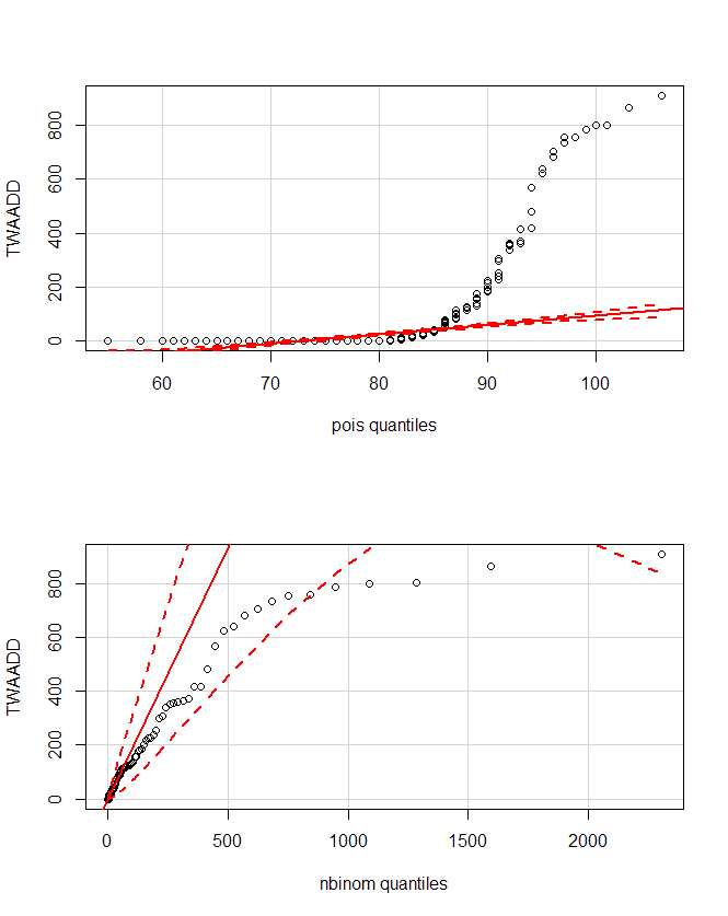
When checking my response variable (the counts of the behaviour) it most likely fits a negative binomial distibution:

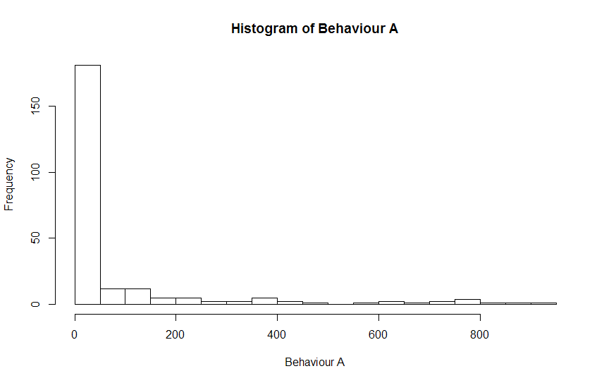
When looking at the data the it has a very high count of zeros (133 out of 240 to be exact)

quantile(Data$ACTW)
  0%    25%    50%    75%   100%
0.00   0.00   0.00  44.75 909.00
The problem I face now is that when I want to fit a negative binomial model with nested random effects with lme4, I come across a convergence error.
This is my Model:
ACTW_Model_CP <- glmer.nb(ACTW ~ Condition + Parent + (1|Nest/Individual) + (1|ACTW_BL),
                          weights = Seen, data = Data, verbose = TRUE)
- ACTW is the Behaviour in question
- Condition is the treatment condition
- Parent is the sex
- Nest is the specific nest/the location
- Individual is the identifier for the individual
- ACTW_BL is the behaviour recorded during baseline observations
- Seen is the amount of time the individual was seen (Zero to one)
Running the model resulted in:
> ACTW_Model_CP <- glmer.nb(ACTW ~ Condition + Parent + (1|Nest/Individual) + (1|ACTW_BL),
+ data = Data, weights = Seen, verbose = TRUE)
theta.ml: iter 0 'theta = 0.830397'
theta.ml: iter1 theta =-0.687164
theta.ml: iter2 theta =-0.0026382
theta.ml: iter3 theta =0.00521452
theta.ml: iter4 theta =0.0102195
theta.ml: iter5 theta =0.0197524
theta.ml: iter6 theta =0.0373503
theta.ml: iter7 theta =0.0683011
theta.ml: iter8 theta =0.118839
theta.ml: iter9 theta =0.192281
theta.ml: iter10 theta =0.280215
theta.ml: iter11 theta =0.354639
theta.ml: iter12 theta =0.387487
theta.ml: iter13 theta =0.391826
theta.ml: iter14 theta =0.39189
th := est_theta(glmer(..)) = 0.3918897
Error in eval(expr, envir, enclos) :
  pwrssUpdate did not converge in (maxit) iterations
In addition: Warning message:
In checkConv(attr(opt, "derivs"), opt$par, ctrl = control$checkConv,  :
  Model failed to converge with max|grad| = 0.017808 (tol = 0.001, component 1)
I have tried to simplify the model, yet I did not manage to get any models calculated. I also tried both optimisers included in lme4.
My question is as follows: Is there a way to model my data in a way that accounts for the amount of time an individual was seen during the experiment?
I'm running lme4 version 1.1-12 in R 3.2.1 under Windows 7 (x86_64-w64-mingw32).

maxit? $\endgroup$control=glmerControl(optCtrl=list(maxfun=2000000))but it still did not reach convergence in thepwrssUpdate (...)TheIn addition:(...)-Warning did go away though $\endgroup$ACTW_BLas a random effect ? $\endgroup$ACTW_BLas a random effect as because I want to correct for the effect that the presence of humans had on the birds' behaviour. $\endgroup$ACTW_BLis a baseline measurement of your outcome variable. I don't see any rationale for treating it as a grouping variable.To be a random effect it should be 1) a factor (ie. not something measured), 2) a sample from a larger population. By treating it as random you are saying that your measurements are clustered within each level of it. $\endgroup$