Why does Latent Dirichlet Allocation seems to work with greedy selection but not with Gibbs sampling?

Question

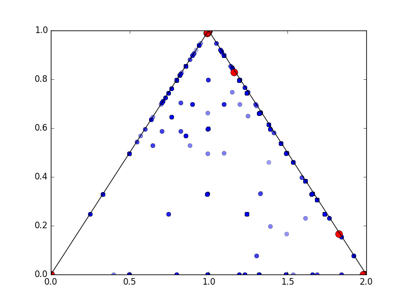
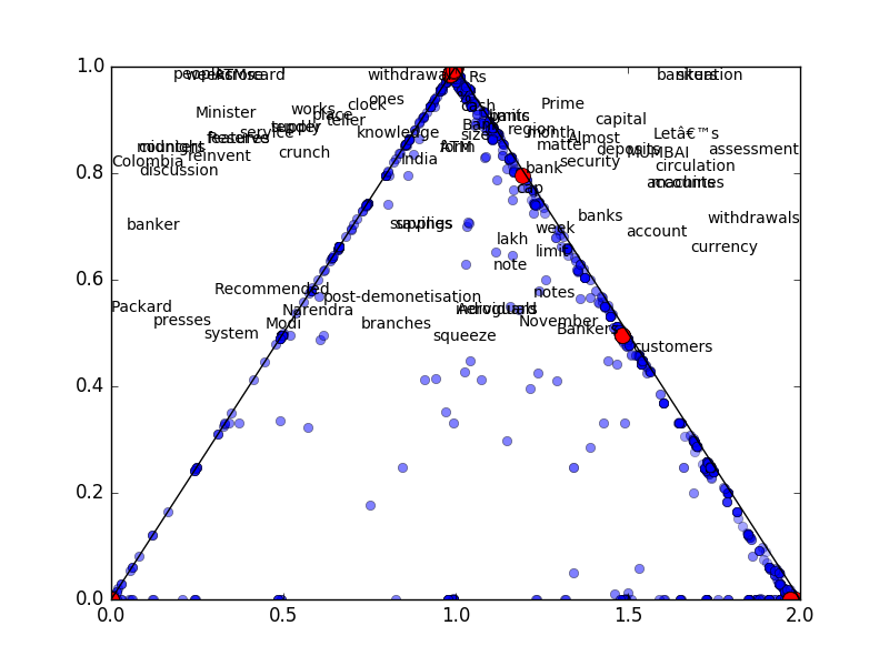
I tried to implement my own LDA program in python, while following this tutorial. When I use gibbs sampling, the program assigns all words to a particular topic on convergence. When I greedily np.argmax assign the topics according to the probability, then program seems to work fine. Is there a problem with the code or my intuition?

import numpy as np
import collections
import matplotlib.pyplot as plt
#import nltk

ITERATIONS = 100
px = [0,1,2]
py = [0,1,0]

n = 50 # Number of documents
k = 3 # Number of topics
v = 100 # Number of distinct words

# Dirichlet parameters
alpha = .01
lamb = .01

# How much each document pertains to a perticular topic
a = np.matrix(np.zeros((n,k)))

# How much each word pertains to a perticular topic
b = np.matrix(np.zeros((k,v)))

# Generate random documents for testing
minLength = 25
maxLength = 50

sentenceLengths = range(int(np.random.uniform(minLength,maxLength)))

# Labeled dataset, each word is replaced with its topic index
topicAssignment = [[int(np.random.uniform(0,k))
           for _ in sentenceLengths]
           for _ in range(n)]

# Labeled dataset, each word is replaced with its bag of words index
wordIndexes = [[int(np.random.uniform(0,v))
           for _ in sentenceLengths]
           for _ in range(n)]

def rouletteArg(vector):
    # Uncomment the next line for greedy
    #return np.argmax(vector)
    vector /= np.sum(vector)
    val = np.random.uniform()
    #print(vector)
    for i in range(len(vector)):
        val -= vector[i]
        if val <= 0:
            return i
    return len(vector)-1

def update(a,b,topicAssignment):
    # Count the number of times words from each topic are used
    # in the document
    for document in range(n):
        occurance = collections.Counter(topicAssignment[document])
        for topic in range(k):        
            a[document,topic] = occurance[topic]
        a[document] /= np.sum(a[document] + alpha)

    # Count the number of times a word is used in a particular topic
    for document in range(n):
        doc = wordIndexes[document]
        for wordIndex in range(len(doc)):
            topic = topicAssignment[document][wordIndex]
            word = wordIndexes[document][wordIndex]
            b[topic,word] += 1

    # Normalize
    for i in range(len(b.T)):
        b.T[i]/= np.sum(b.T[i] + lamb)

    # Update the assignment of topics
    for document in range(n):
        for wordIndex in range(len(topicAssignment[document])):
            vec = np.zeros(k)
            for topic in range(k):
                word = wordIndexes[document][wordIndex]
                vec[topic] = (a[document,topic] + alpha) * (b[topic,word] + lamb)
            topicAssignment[document][wordIndex] = rouletteArg(vec)

    return a,b,topicAssignment

a,b,topicAssignment = update(a,b,topicAssignment)

costs = np.zeros(ITERATIONS)
for iteration in range(ITERATIONS):
    lastA = a.copy()
    lastB = b.copy()
    a,b,topicAssignment = update(a,b,topicAssignment)
    cost = np.sum(np.abs(a-lastA)) + np.sum(np.abs(b-lastB))
    costs[iteration] = cost

    if cost <= 1e-7:
        break

    plt.figure(1)
    x = a * np.matrix(px).T
    y = a * np.matrix(py).T
    plt.plot(x,y,'bo',alpha=((1.0-iteration/ITERATIONS)*.5))

    plt.figure(2)
    x = b.T * np.matrix(px).T
    y = b.T * np.matrix(py).T
    plt.plot(x,y,'bo',alpha=((1.0-iteration/ITERATIONS)*.5))

    print(iteration,cost)

plt.figure(1)
fig = plt.gcf()
fig.canvas.set_window_title('Document Distribution')
x = a * np.matrix(px).T
y = a * np.matrix(py).T
plt.plot(x,y,'ro',ms=10)
plt.plot(px,py,'k-')

plt.figure(2)
fig = plt.gcf()
fig.canvas.set_window_title('Word Distribution')
x = b.T * np.matrix(px).T
y = b.T * np.matrix(py).T
plt.plot(x,y,'ro',ms=10)
plt.plot(px,py,'k-')

plt.figure(3)
fig = plt.gcf()
fig.canvas.set_window_title('Cost Function')
plt.plot(costs)
plt.show()

The the lighter shades of blue are earlier iterations and darker are later iterations. The red circles are the convergence.

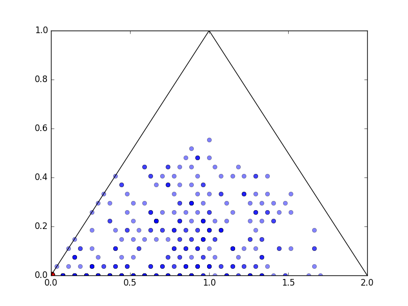Fig 1. Document allocation using gibbs 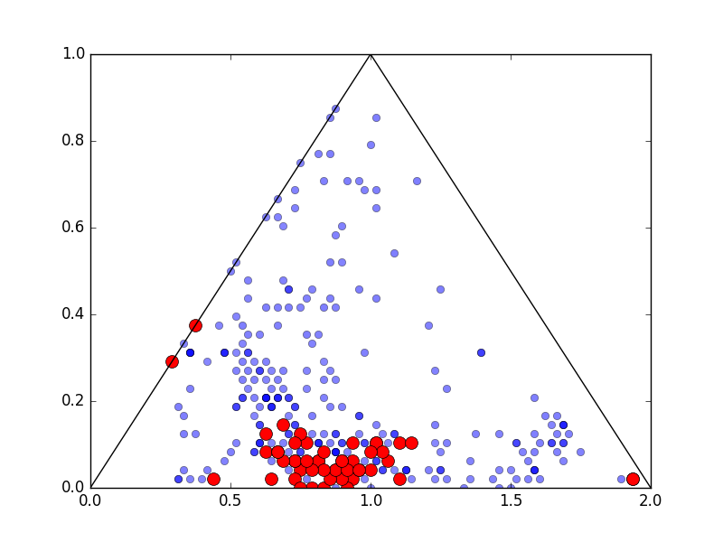Fig 2. Document allocation using greedy 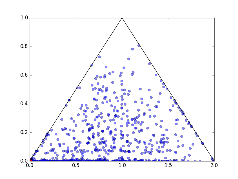Fig 3. Word allocation using gibbs 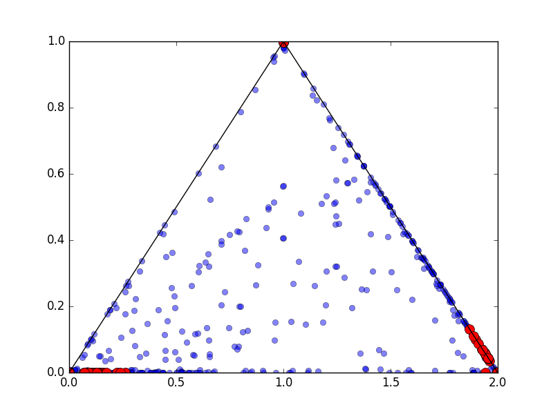Fig 4. Word allocation using greedy

Answer 1

I tried it on some actual data and got similar results. Then I read this post. The large number of uninformative words like The,at,a etc confuses the LDA because they are everywhere. I used nltk.pos_tag to remove all words except for nouns.

Fig 1. Document Allocation

Fig 2. Word Allocation

As far as the question goes, "why did the greedy approach seem to work?", I think since the uniform distribution scatters the words uniformly in the triangle, the words simply moved to its closest vertex and stayed there because it is the local optima. The gibbs sampling nudged them out of their local optima and they all collapsed together.