37
$\begingroup$

I have data on movement behaviours (time spent sleeping, sedentary, and doing physical activity) that sums to approximately 24 (as in hours per day). I want to create a variable that captures the relative time spent in each of these behaviours - I've been told that an isometric log-ratio transformation would accomplish this.

It looks like I should use the ilr function in R, but can't find any actual examples with code. Where do I start?

The variables I have are time spent sleeping, average sedentary time, average average light physical activity, average moderate physical activity, and average vigorous physical activity. Sleep was self-reported, while the others are averages from valid days of accelerometer data. So for these variables, cases do not sum to exactly 24.

My guess: I'm working in SAS, but it looks like R will be much easier to use for this part. So first import data with only the variables of interest. Then use acomp() function. Then I can't figure out the syntax for the ilr() function. Any help would be much appreciated.

$\endgroup$

3 Answers 3

47
$\begingroup$

The ILR (Isometric Log-Ratio) transformation is used in the analysis of compositional data. Any given observation is a set of positive values summing to unity, such as the proportions of chemicals in a mixture or proportions of total time spent in various activities. The sum-to-unity invariant implies that although there may be $k\ge 2$ components to each observation, there are only $k-1$ functionally independent values. (Geometrically, the observations lie on a $k-1$-dimensional simplex in $k$-dimensional Euclidean space $\mathbb{R}^k$. This simplicial nature is manifest in the triangular shapes of the scatterplots of simulated data shown below.)

Typically, the distributions of the components become "nicer" when log transformed. This transformation can be scaled by dividing all values in an observation by their geometric mean before taking the logs. (Equivalently, the logs of the data in any observation are centered by subtracting their mean.) This is known as the "Centered Log-Ratio" transformation, or CLR. The resulting values still lie within a hyperplane in $\mathbb{R}^k$, because the scaling causes the sum of the logs to be zero. The ILR consists of choosing any orthonormal basis for this hyperplane: the $k-1$ coordinates of each transformed observation become its new data. Equivalently, the hyperplane is rotated (or reflected) to coincide with the plane with vanishing $k^\text{th}$ coordinate and one uses the first $k-1$ coordinates. (Because rotations and reflections preserve distance they are isometries, whence the name of this procedure.)

Tsagris, Preston, and Wood state that "a standard choice of [the rotation matrix] $H$ is the Helmert sub-matrix obtained by removing the first row from the Helmert matrix."

The Helmert matrix of order $k$ is constructed in a simple manner (see Harville p. 86 for instance). Its first row is all $1$s. The next row is one of the the simplest that can be made orthogonal to the first row, namely $(1, -1, 0, \ldots, 0)$. Row $j$ is among the simplest that is orthogonal to all preceding rows: its first $j-1$ entries are $1$s, which guarantees it is orthogonal to rows $2, 3, \ldots, j-1$, and its $j^\text{th}$ entry is set to $1-j$ to make it orthogonal to the first row (that is, its entries must sum to zero). All rows are then rescaled to unit length.

Here, to illustrate the pattern, is the $4\times 4$ Helmert matrix before its rows have been rescaled:

$$\pmatrix{1&1&1&1 \\ 1&-1&0&0 \\ 1&1&-2&0 \\ 1&1&1&-3}.$$

(Edit added August 2017) One particularly nice aspect of these "contrasts" (which are read row by row) is their interpretability. The first row is dropped, leaving $k-1$ remaining rows to represent the data. The second row is proportional to the difference between the second variable and the first. The third row is proportional to the difference between the third variable and the first two. Generally, row $j$ ($2\le j \le k$) reflects the difference between variable $j$ and all those that precede it, variables $1, 2, \ldots, j-1$. This leaves the first variable $j=1$ as a "base" for all contrasts. I have found these interpretations helpful when following the ILR by Principal Components Analysis (PCA): it enables the loadings to be interpreted, at least roughly, in terms of comparisons among the original variables. I have inserted a line into the R implementation of ilr below that gives the output variables suitable names to help with this interpretation. (End of edit.)

Since R provides a function contr.helmert to create such matrices (albeit without the scaling, and with rows and columns negated and transposed), you don't even have to write the (simple) code to do it. Using this, I implemented the ILR (see below). To exercise and test it, I generated $1000$ independent draws from a Dirichlet distribution (with parameters $1,2,3,4$) and plotted their scatterplot matrix. Here, $k=4$.
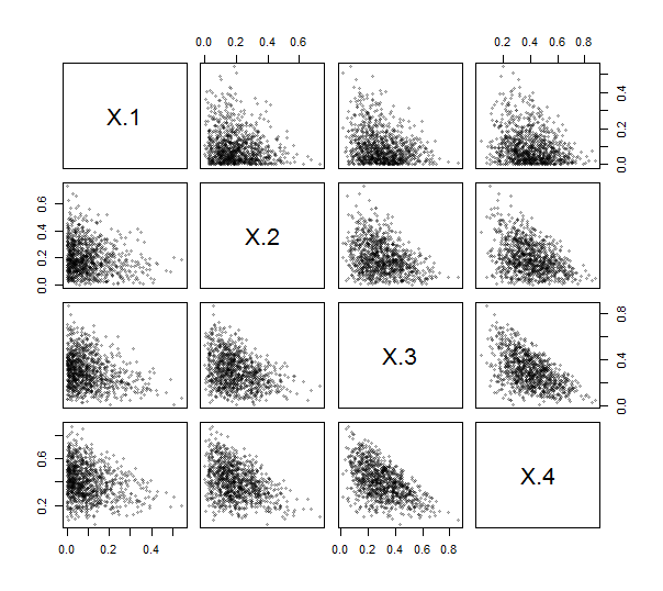
Figure_1

The points all clump near the lower left corners and fill triangular patches of their plotting areas, as is characteristic of compositional data.

Their ILR has just three variables, again plotted as a scatterplot matrix:

Figure_2

This does indeed look nicer: the scatterplots have acquired more characteristic "elliptical cloud" shapes, better amenable to second-order analyses such as linear regression and PCA.

Tsagris et al. generalize the CLR by using a Box-Cox transformation, which generalizes the logarithm. (The log is a Box-Cox transformation with parameter $0$.) It is useful because, as the authors (correctly IMHO) argue, in many applications the data ought to determine their transformation. For these Dirichlet data a parameter of $1/2$ (which is halfway between no transformation and a log transformation) works beautifully:
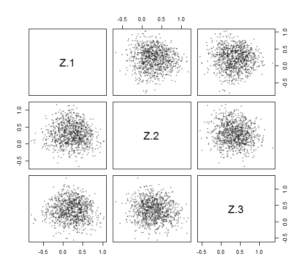
Figure_3

"Beautiful" refers to the simple description this picture permits: instead of having to specify the location, shape, size, and orientation of each point cloud, we need only observe that (to an excellent approximation) all the clouds are circular with similar radii. In effect, the CLR has simplified an initial description requiring at least 16 numbers into one that requires only 12 numbers and the ILR has reduced that to just four numbers (three univariate locations and one radius), at a price of specifying the ILR parameter of $1/2$--a fifth number. When such dramatic simplifications happen with real data, we usually figure we're on to something: we have made a discovery or achieved an insight.


This generalization is implemented in the ilr function below. The command to produce these "Z" variables was simply

z <- ilr(x, 1/2)

One advantage of the Box-Cox transformation is its applicability to observations that include true zeros: it is still defined provided the parameter is positive.

References

Michail T. Tsagris, Simon Preston and Andrew T.A. Wood, A data-based power transformation for compositional data. arXiv:1106.1451v2 [stat.ME] 16 Jun 2011.

David A. Harville, Matrix Algebra From a Statistician's Perspective. Springer Science & Business Media, Jun 27, 2008.


Here is the R code.

#
# ILR (Isometric log-ratio) transformation.
# `x` is an `n` by `k` matrix of positive observations with k >= 2.
#
ilr <- function(x, p=0) {
  y <- log(x)
  if (p != 0) y <- (exp(p * y) - 1) / p       # Box-Cox transformation
  y <- y - rowMeans(y, na.rm=TRUE)            # Recentered values
  k <- dim(y)[2]
  H <- contr.helmert(k)                       # Dimensions k by k-1
  H <- t(H) / sqrt((2:k)*(2:k-1))             # Dimensions k-1 by k
  if(!is.null(colnames(x)))                   # (Helps with interpreting output)
    colnames(z) <- paste0(colnames(x)[-1], ".ILR")
  return(y %*% t(H))                          # Rotated/reflected values
}
#
# Specify a Dirichlet(alpha) distribution for testing.
#
alpha <- c(1,2,3,4)
#
# Simulate and plot compositional data.
#
n <- 1000
k <- length(alpha)
x <- matrix(rgamma(n*k, alpha), nrow=n, byrow=TRUE)
x <- x / rowSums(x)
colnames(x) <- paste0("X.", 1:k)
pairs(x, pch=19, col="#00000040", cex=0.6)
#
# Obtain the ILR.
#
y <- ilr(x)
colnames(y) <- paste0("Y.", 1:(k-1))
#
# Plot the ILR.
#
pairs(y, pch=19, col="#00000040", cex=0.6)
$\endgroup$
25
  • 2
    $\begingroup$ @Alex I don't understand what you mean by "spurious" correlations. Yes, the variables must be dependent--but the job of PCA is to help you characterize and quantify those dependencies. Note, too, that the sum of the CLRs is not constant (even though the CLRs are based on values that sum to unity). $\endgroup$
    – whuber
    Commented Nov 2, 2017 at 18:51
  • 2
    $\begingroup$ @Alex Sure--that's why I use scatterplots in this answer to illustrate the ILR! $\endgroup$
    – whuber
    Commented Nov 3, 2017 at 16:30
  • 3
    $\begingroup$ @Alex That's an interesting quotation. It appears to reflect a philosophy that flies in the face of EDA (among other things), which suggests that when one can find a re-expression of variables that produces useful or informative relationships, that is a good thing, not a problem. Proponents of EDA (like John Tukey) argue that the form in which data are originally expressed is not necessarily the form in which they should be analyzed, whereas this quotation implicitly supposes just the opposite. I'll leave it to you to decide which is the more useful approach. $\endgroup$
    – whuber
    Commented Nov 6, 2017 at 14:13
  • 2
    $\begingroup$ @Eli That comment was intended to refer to the generalized CLR. As I wrote in the body of this answer, "the scaling causes the sum of the logs to be zero." $\endgroup$
    – whuber
    Commented Jun 18, 2018 at 23:55
  • 3
    $\begingroup$ @Bart the $k=3$ triangle has three natural coordinates, but only two dimensions, because the coordinates are redundant. $\endgroup$
    – whuber
    Commented Feb 28, 2020 at 0:43
8
$\begingroup$

For your use case, it is probably ok to just scale everything down to one. The fact the numbers don't add up exactly to 24 will add a little extra noise to the data, but it shouldn't mess things up that much.

As @whuber correctly stated, since we are dealing with proportions, we have to account for dependencies between the variables (since they add up to one). The ilr transform appropriately deals with this, since it transforms the variables into $\mathbb{R}^{D-1}$ for $D$ proportions.

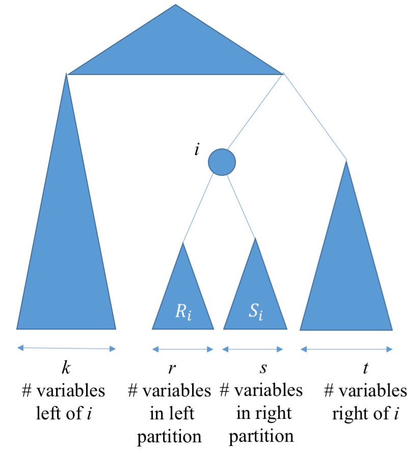
All of the technical details aside, it is important to know how to properly interpret the ilr transformed data. In the end, the ilr transform just refers to the log ratios of groups. But it defines it with respect to some predefined hierarchy. If you define a hierarchy like as follows

enter image description here

each transformed variable can be calculated as

$b_i = \sqrt{\frac{rs}{r + s}}\ln \frac{g(R_i)}{g(S_i)}$

where $i$ represents an internal node in the hierarchy, $R_i$ defines one partition of variables corresponding to $i$, $S_i$ defines the other partition of variables corresponding to $i$ and $g(...)$ refers to the geometric mean. These transformed variables are also known as balances.

So the next question is, how do you define your hierarchy of variables? This is really up to you, but if you have three variables, there aren't too many combinations to mess with. For instance, you could just define the hierarchy to be

                        /-A
            /(A|B)-----|
-(AB|C)----|            \-B
           |
            \-C

where A represents the time spent sleeping, B represents time spent with sedentary, C represents time spent doing physical activity (A|B) represents the normalized log ratio between $A$ $B$ (i.e. $\frac{1}{\sqrt{2}}\ln \frac{A}{B}$ ), and $(AB|C)$ refers to the normalized log ratio between $A$, $B$ and $C$ (i.e. $\frac{\sqrt{2}}{\sqrt{3}} \ln \frac{AB}{C}$). If there are many variables, I check out some of the work done with principal balances

But going back to your original question, how can you use this information to actually perform the ilr transformation?

If you are using R, I'd checkout the compositions package

To use that package, you'll need to understand how to create a sequential binary partition (SBP), which is how you define the hierarchy. For the hierarchy defined above, you can represent the SBP with the following matrix.

        A  B  C
(A|B)   1 -1  0
(AB|C)  1  1 -1

where the positive values represent the variables in the numerator, the negative values represent the variables in the denominator, and zeros represent the absence of that variable in the balance. You can build the orthonormal basis using balanceBase from the SBP that you defined.
Once you have this you should be able to pass in your table of proportions along with the basis that you calculated above.

I'd check out this reference for the original definition of balances

$\endgroup$
5
$\begingroup$

The above posts answer the question about how to construct an ILR basis and get your ILR balances. To add to this, the choice of which basis can ease the interpretation of your results.

You may be interested in a partition the following partition:

(1) (sleeping,sedentary|physical_activity) (2) (sleeping|sedentary).

Since you have three parts in your composition, you will obtain two ILR balances to analyze. By setting up the partition as above, you can obtain balances corresponding to "active or not" (1) and "which form of inactivity" (2).

If you analyze each ILR balance separately, for instance performing regression against time-of-day or time-of-year to see if there are any changes, you can interpret the results in terms of changes in "active or not" and changes in "which form of inactivity".

If, on the other hand, you will perform techniques like PCA which obtain a new basis in ILR space, your results will not depend on your choice of partition. This is because your data exist in CLR-space, the D-1 plane orthogonal to the one-vector, and the ILR balances are different choices of unit-norm axes to describe the data's position on the CLR plane.

$\endgroup$

Your Answer

By clicking “Post Your Answer”, you agree to our terms of service and acknowledge you have read our privacy policy.

Not the answer you're looking for? Browse other questions tagged or ask your own question.