Fitting simple (binomial) model in PyMC - slow convergence

Question

I am trying to use pymc to estimate parameters for a model. As I am not familiar with the methodology I first generated the data myself and tried to derive the posterior distribution using pymc.

The data consists of a (time-) series of the number of missed payments $D$ for each quarter. For each quarter, the probability of a client missing a payment is a random variable, $p(x,\alpha)$, that depends on two parameters, $\alpha$ which is an unknown constant (in time) that I'm trying to estimate, and $x \sim \mathcal{N}(0,1)$, which is a random variable and drawn for each quarter.

Edit: for clarity, the function $p(x,\alpha)$ below describes the probability of a client to miss a payment. This probability is normally 3% per quarter but fluctuates a bit however, based on a correlation between clients ($\alpha$) and a random number. Please note each quarter is independent from the other. Only $x$ makes this a random variable. I have coded this as a deterministic in PyMC as its value it determined completely by $\alpha$ and $x$.

The actual probability of missing a payment in a quarter is described by the following function:

$$p(x,\alpha) = \Phi \left( \frac{ \Phi^{-1}(rate) - \alpha x }{\sqrt{1-\alpha^2}}\right) $$

where $\Phi$ is the normal cumulative distribution function and $\Phi^{-1}$ its inverse.

To generate a data sample for 50 quarters I have used this code (with the sample $\alpha = 0.37$ ).

sample_alpha = 0.37
const_z = 0.03 # basis prob of missing payment (3%)
nr_clients = 10000
nr_quarters = 50


Xs = np.random.normal(loc=0.0, scale=1.0,size=nr_quarters)

def p(x,a):
    return sp.norm.cdf( (sp.norm.ppf(const_z) - sample_alpha*Xs)/(np.sqrt(1-sample_alpha*sample_alpha)) )

sample_mp = np.random.binomial(n=nr_clients, p=p(Xs,sample_alpha))

py.xlabel('quarter')
py.ylabel('nr of missed payments')
py.plot(sample_mp)

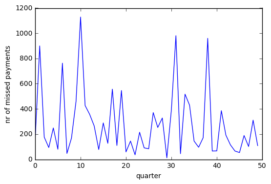
Below is shown a random realization of this process. To give more insight: every quarter the random variable $x$ and the actual $\alpha$ produce a certain probability of missing a payment. What is shown below for each quarter is then a drawing from a random binomial variable where the probability of success is this probability of missing a payment.

Now I'm trying to estimate the posterior distribution of $\alpha$ from this realization. I am using the following pymc code:

xfactor = pm.Normal('xfactor', mu=0, tau=1/(1*1), size = sample_mp.shape[0])

alpha = pm.Uniform("alpha", 0.01,0.99)

@pm.deterministic
def P(x=xfactor,a=alpha):
    return sp.norm.cdf( (sp.norm.ppf(const_z) - a*x)/(np.sqrt(1-a*a)) )


missed_payments = pm.Binomial('defaults',n=10000,p=P, value=sample_mp,observed=True)
model = pm.Model([xfactor, alpha, P, missed_payments])

And then try to run it to get some feeling of what is going on (I haven't set burn-in and thinning at this point):

mcmc = pm.MCMC(model)
mcmc.sample(30000)
pm.Matplot.plot(mcmc)

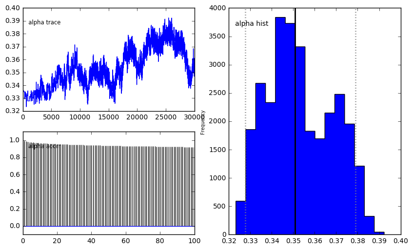
The results look like this:

When I increase the nr of samples the plot is similar. I understand from this that $\alpha$ doesn't seem to converge, and the autocorrelation plot looks problematic too, but I am uncertain how to resolve the issue.

Answer 1

Here is my shot at the problem in PyMC3. I can be wrong how the model is built, so please correct me where I am wrong.

The data are 50 observations (50 binomial draws) that are i.i.d. This assumptions is strong one.

I set the true parameter value (p_true=0.37) and set number of Bernoulli trials to 10,000. With these parameters set, I draw (K=50) samples from the Binomial distribution.

import pymc3 as pm
import matplotlib.pyplot as plt

from scipy.stats import binom

p_true = 0.37
n = 10000
K = 50

X = binom.rvs( n=n, p=p_true, size=K )
print( X )

model = pm.Model()

with model:
    p = pm.Beta( 'p', alpha=2, beta=2 )
    y_obs = pm.Binomial( 'y_obs', p=p, n=n, observed=X )
    step = pm.Metropolis()
    trace = pm.sample( 10000, step=step, progressbar=True )

pm.traceplot( trace )
plt.show()