9
$\begingroup$

We have a data set with two covariates and a categorical grouping variable and want to know if there are significant differences between the slope or intercept among the covariates associated with the different grouping variables. We've used anova() and lm() to compare the fits of three different models: 1) with a single slope and intercept, 2) with different intercepts for each group, and 3) with a slope and an intercept for each group. According to the anova() general linear test, the second model is the most appropriate of the three, there is a significant improvement to the model by including a separate intercept for each group. However, when we look at the 95% confidence intervals for these intercepts -- they all overlap, suggesting there aren't significant differences between the intercepts. How can these two results be reconciled? We thought another way of interpreting the results of the model-selection method was that there has to be at least one significant difference among the intercepts... but perhaps this is not correct?

Below is the R code to replicate this analysis. We've used the dput() function so you can work with exactly the same data we're grappling with.

# Begin R Script
# > dput(data)
structure(list(Head = c(1.92, 1.93, 1.79, 1.94, 1.91, 1.88, 1.91, 
1.9, 1.97, 1.97, 1.95, 1.93, 1.95, 2, 1.87, 1.88, 1.97, 1.88, 
1.89, 1.86, 1.86, 1.97, 2.02, 2.04, 1.9, 1.83, 1.95, 1.87, 1.93, 
1.94, 1.91, 1.96, 1.89, 1.87, 1.95, 1.86, 2.03, 1.88, 1.98, 1.97, 
1.86, 2.04, 1.86, 1.92, 1.98, 1.86, 1.83, 1.93, 1.9, 1.97, 1.92, 
2.04, 1.92, 1.9, 1.93, 1.96, 1.91, 2.01, 1.97, 1.96, 1.76, 1.84, 
1.92, 1.96, 1.87, 2.1, 2.17, 2.1, 2.11, 2.17, 2.12, 2.06, 2.06, 
2.1, 2.05, 2.07, 2.2, 2.14, 2.02, 2.08, 2.16, 2.11, 2.29, 2.08, 
2.04, 2.12, 2.02, 2.22, 2.22, 2.2, 2.26, 2.15, 2, 2.24, 2.18, 
2.07, 2.06, 2.18, 2.14, 2.13, 2.2, 2.1, 2.13, 2.15, 2.25, 2.14, 
2.07, 1.98, 2.16, 2.11, 2.21, 2.18, 2.13, 2.06, 2.21, 2.08, 1.88, 
1.81, 1.87, 1.88, 1.87, 1.79, 1.99, 1.87, 1.95, 1.91, 1.99, 1.85, 
2.03, 1.88, 1.88, 1.87, 1.85, 1.94, 1.98, 2.01, 1.82, 1.85, 1.75, 
1.95, 1.92, 1.91, 1.98, 1.92, 1.96, 1.9, 1.86, 1.97, 2.06, 1.86, 
1.91, 2.01, 1.73, 1.97, 1.94, 1.81, 1.86, 1.99, 1.96, 1.94, 1.85, 
1.91, 1.96, 1.9, 1.98, 1.89, 1.88, 1.95, 1.9, 1.94, NA, 1.84, 
1.83, 1.84, 1.96, 1.74, 1.91, 1.84, 1.88, 1.83, 1.93, 1.78, 1.88, 
1.93, 2.15, 2.16, 2.23, 2.09, 2.36, 2.31, 2.25, 2.29, 2.3, 2.04, 
2.22, 2.19, 2.25, 2.31, 2.3, 2.28, 2.25, 2.15, 2.29, 2.24, 2.34, 
2.2, 2.24, 2.17, 2.26, 2.18, 2.17, 2.34, 2.23, 2.36, 2.31, 2.13, 
2.2, 2.27, 2.27, 2.2, 2.34, 2.12, 2.26, 2.18, 2.31, 2.24, 2.26, 
2.15, 2.29, 2.14, 2.25, 2.31, 2.13, 2.09, 2.24, 2.26, 2.26, 2.21, 
2.25, 2.29, 2.15, 2.2, 2.18, 2.16, 2.14, 2.26, 2.22, 2.12, 2.12, 
2.16, 2.27, 2.17, 2.27, 2.17, 2.3, 2.25, 2.17, 2.27, 2.06, 2.13, 
2.11, 2.11, 1.97, 2.09, 2.06, 2.11, 2.09, 2.08, 2.17, 2.12, 2.13, 
1.99, 2.08, 2.01, 1.97, 1.97, 2.09, 1.94, 2.06, 2.09, 2.04, 2, 
2.14, 2.07, 1.98, 2, 2.19, 2.12, 2.06, 2, 2.02, 2.16, 2.1, 1.97, 
1.97, 2.1, 2.02, 1.99, 2.13, 2.05, 2.05, 2.16, 2.02, 2.02, 2.08, 
1.98, 2.04, 2.02, 2.07, 2.02, 2.02, 2.02), Site = structure(c(2L, 
2L, 2L, 2L, 2L, 2L, 2L, 2L, 2L, 2L, 2L, 2L, 2L, 2L, 2L, 2L, 2L, 
5L, 5L, 5L, 5L, 5L, 5L, 5L, 5L, 5L, 5L, 5L, 5L, 5L, 5L, 5L, 5L, 
5L, 5L, 5L, 3L, 3L, 3L, 3L, 3L, 3L, 3L, 3L, 3L, 3L, 3L, 3L, 3L, 
3L, 3L, 3L, 3L, 3L, 3L, 3L, 3L, 3L, 3L, 3L, 3L, 3L, 3L, 3L, 3L, 
3L, 3L, 3L, 3L, 3L, 3L, 3L, 4L, 4L, 4L, 4L, 4L, 4L, 4L, 4L, 4L, 
4L, 4L, 4L, 4L, 4L, 4L, 4L, 4L, 4L, 4L, 4L, 4L, 4L, 4L, 4L, 4L, 
4L, 1L, 1L, 1L, 1L, 1L, 1L, 1L, 1L, 1L, 1L, 1L, 1L, 1L, 1L, 1L, 
1L, 1L, 1L, 1L, 1L, 1L, 1L, 1L, 1L, 1L, 1L, 1L, 1L, 1L, 1L, 1L, 
1L, 1L, 1L, 6L, 6L, 6L, 6L, 6L, 6L, 6L, 6L, 6L, 6L, 6L, 6L, 6L, 
6L, 6L, 6L, 6L, 6L, 6L, 6L), .Label = c("ANZ", "BC", "DV", "MC", 
"RB", "WW"), class = "factor"), Leg = c(2.38, 2.45, 2.22, 2.23, 
2.26, 2.32, 2.28, 2.17, 2.39, 2.27, 2.42, 2.33, 2.31, 2.32, 2.25, 
2.27, 2.38, 2.28, 2.33, 2.24, 2.21, 2.22, 2.42, 2.23, 2.36, 2.2, 
2.28, 2.23, 2.33, 2.35, 2.36, 2.26, 2.26, 2.3, 2.23, 2.31, 2.27, 
2.23, 2.37, 2.27, 2.26, 2.3, 2.33, 2.34, 2.27, 2.4, 2.22, 2.25, 
2.28, 2.33, 2.26, 2.32, 2.29, 2.31, 2.37, 2.24, 2.26, 2.36, 2.32, 
2.32, 2.15, 2.2, 2.29, 2.37, 2.26, 2.24, 2.23, 2.24, 2.26, 2.18, 
2.11, 2.23, 2.31, 2.25, 2.15, 2.3, 2.33, 2.35, 2.21, 2.36, 2.27, 
2.24, 2.35, 2.24, 2.33, 2.32, 2.24, 2.35, 2.36, 2.39, 2.28, 2.36, 
2.19, 2.27, 2.39, 2.23, 2.29, 2.32, 2.3, 2.32, NA, 2.25, 2.24, 
2.21, 2.37, 2.21, 2.21, 2.27, 2.27, 2.26, 2.19, 2.2, 2.25, 2.25, 
2.25, NA, 2.24, 2.17, 2.2, 2.2, 2.18, 2.14, 2.17, 2.27, 2.28, 
2.27, 2.29, 2.23, 2.25, 2.33, 2.22, 2.29, 2.19, 2.15, 2.24, 2.24, 
2.26, 2.25, 2.09, 2.27, 2.18, 2.2, 2.25, 2.24, 2.18, 2.3, 2.26, 
2.18, 2.27, 2.12, 2.18, 2.33, 2.13, 2.28, 2.23, 2.16, 2.2, 2.3, 
2.31, 2.18, 2.33, 2.29, 2.26, 2.21, 2.22, 2.27, 2.32, 2.24, 2.25, 
2.17, 2.2, 2.26, 2.27, 2.24, 2.25, 2.09, 2.25, 2.21, 2.24, 2.21, 
2.22, 2.13, 2.24, 2.21, 2.3, 2.34, 2.35, 2.32, 2.46, 2.43, 2.42, 
2.41, 2.32, 2.25, 2.33, 2.19, 2.45, 2.32, 2.4, 2.38, 2.35, 2.39, 
2.29, 2.35, 2.43, 2.29, 2.33, 2.31, 2.28, 2.38, 2.32, 2.43, 2.27, 
2.4, 2.37, 2.27, 2.41, 2.32, 2.38, 2.23, 2.33, 2.21, 2.34, 2.19, 
2.34, 2.35, 2.35, 2.31, 2.33, 2.41, 2.53, 2.39, 2.17, 2.16, 2.38, 
2.34, 2.33, 2.33, 2.29, 2.43, 2.28, 2.34, 2.38, 2.3, 2.29, 2.43, 
2.36, 2.24, 2.35, 2.38, 2.4, 2.36, 2.42, 2.28, 2.45, 2.33, 2.32, 
2.33, 2.31, 2.44, 2.37, 2.4, 2.35, 2.33, 2.31, 2.36, 2.43, 2.38, 
2.4, 2.38, 2.46, 2.33, 2.38, 2.23, 2.24, 2.39, 2.36, 2.19, 2.32, 
2.37, 2.39, 2.34, 2.39, 2.23, 2.25, 2.29, 2.39, 2.35, NA, 2.28, 
2.35, 2.38, 2.34, 2.17, 2.29, NA, 2.26, NA, NA, NA, 2.24, 2.33, 
2.23, 2.28, 2.29, 2.23, 2.2, 2.27, 2.31, 2.31, 2.26, 2.28)), .Names = c("Head", 
"Site", "Leg"), class = "data.frame", row.names = c(NA, -312L
)) 

# plot graph
library(ggplot2)

qplot(Head, Leg, 
    color=Site, 
    data=data) + 
        stat_smooth(method="lm", alpha=0.2) + 
        theme_bw()
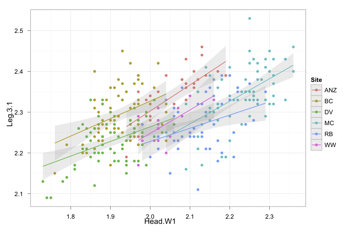
enter image description here

# create linear models
lm.1 <- lm(Leg ~ Head, data)
lm.2 <- lm(Leg ~ Head + Site, data)
lm.3 <- lm(Leg ~ Head*Site, data)

# evaluate linear models
anova(lm.1, lm.2, lm.3)
anova(lm.1, lm.2)

# > anova(lm.1, lm.2)
# Analysis of Variance Table
# Model 1: Leg.3.1 ~ Head.W1
# Model 2: Leg.3.1 ~ Head.W1 + Site
  # Res.Df     RSS Df Sum of Sq     F    Pr(>F)    
# 1    302 1.25589                                 
# 2    297 0.91332  5   0.34257 22.28 < 2.2e-16 ***


# examining the multiple-intercepts model (lm.2)
summary(lm.2)
coef(lm.2)
confint(lm.2)

# extracting the intercepts
intercepts <- coef(lm.2)[c(1, 3:7)]
intercepts.1 <- intercepts[1]
intercepts <- intercepts.1 + intercepts
intercepts[1] <- intercepts.1
intercepts

# extracting the confidence intervals
ci <- confint(lm.2)[c(1, 3:7),]
ci[2:6,] <- ci[2:6,] + confint(lm.2)[1,]
ci[,1]

# putting everything together in a dataframe
labels <- c("ANZ", "BC", "DV", "MC", "RB", "WW")
ci.dataframe <- data.frame(Site=labels, Intercept=intercepts, CI.low = ci[,1], CI.high = ci[,2])
ci.dataframe

# plotting intercepts and 95% CI
qplot(Site, Intercept, geom=c("point", "errorbar"), ymin=CI.low, ymax=CI.high, data=ci.dataframe, ylab="Intercept & 95% CI")
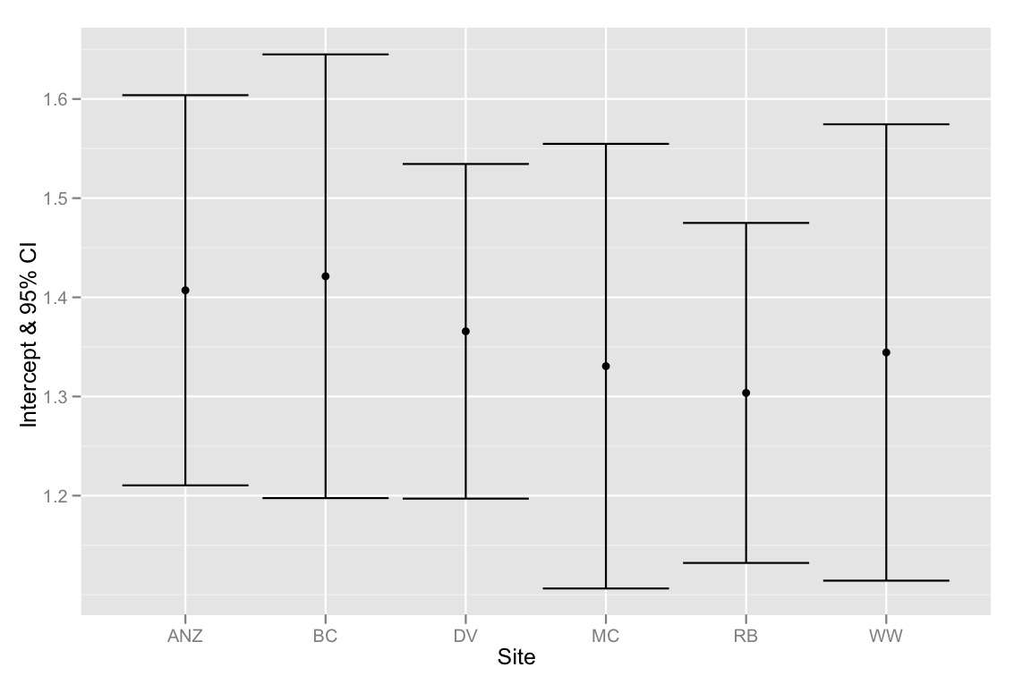
ancova intercepts

Just to summarize -- the problem is that the 95% CIs for the intercepts all overlap, but the model selection method suggests that the best model is one that fits different intercepts. So I'm inclined to think either our model selection method is flawed or the 95% CIs for the intercept estimates were calculated incorrectly. Any thoughts would be greatly appreciated!

$\endgroup$
1
  • 1
    $\begingroup$ Your statistical terminology is confused. You are conflating group means with "intercepts". Not really a coding issue. Suggesting to moderators that it be moved to stats.exchange. $\endgroup$
    – DWin
    Commented Apr 13, 2012 at 13:09

5 Answers 5

11
$\begingroup$

Remember that the difference between significant and non-significant is not (always) statistically significant

Now, more to the point of your question, model 1 is called pooled regression, and model 2 unpooled regression. As you noted, in pooled regression, you assume that the groups aren't relevant, which means that the variance between groups is set to zero.

In the unpooled regression, with an intercept per group, you set the variance to infinity.

In general, I'd favor an intermediate solution, which is a hierarchical model or partial pooled regression (or shrinkage estimator). You can fit this model in R with the lmer4 package.

Finally, take a look at this paper by Gelman, in which he argues why hierarchical models helps with the multiple comparisons problems (in your case, are the coefficients per group different? How do we correct a p-value for multiple comparisons).

For instance, in your case,

library(lme4)
summary(lmer( leg ~ head + (1 | site)) # varying intercept model

If you want to fit a varying-intercept, varying slope (the third model), just run

summary(lmer( leg ~ head + (1 | site) + (0+head|site) )) # varying intercept, varying-slope model

Then you can take a look at the group variance and see if it's different from zero (the pooled regression isn't the better model) and far from infinity (unpooled regression).

update: After the comments (see below), I decided to expand my answer.

The purpose of a hierarchical model, specially in cases like this, is to model the variation by groups (in this case, Sites). So, instead of running an ANOVA to test if a model is different from another, I'd take a look at the predictions of my model and see if the predictions by group is better in the hierarchical models vs the pooled regression (classical regression).

Now, I ran my sugestions above and foudn that

ranef(lmer( leg ~ head + (1 | site) + (0+head|site) )

Would return zero as estimates of varying slope (varying effect of head by site). then I ran

ranef(lmer( leg ~ head + (head| site))

And I got a non-zero estimates for the varying effect of head. I don't know yet why this happened, since it's the first time I found this. I'm really sorry for this problem, but, in my defense, I just followed the specification outlined in the help of the lmer function. (See the example with the data sleepstudy). I'll try to understand what's happening and I'll report here when (if) I understand what's happening.

$\endgroup$
4
  • $\begingroup$ Thanks @manoel-galdino - Is it correct to conclude from these results that since the variance associated with Site here is not sig. different from 0, then this factor is not significant in the model? Random effects: Groups Name Variance Std.Dev. Site (Intercept) 0.0019094 0.043697 Residual 0.0030755 0.055457 $\endgroup$ Commented Apr 17, 2012 at 17:17
  • $\begingroup$ Also @manoel-galdino, could you help me to interpret this part of the model in english? (0+head|site) $\endgroup$ Commented Apr 17, 2012 at 17:23
  • $\begingroup$ @JamesWaters, yep, since site is not significantly different from 0, variation among sites is not that important. $\endgroup$ Commented Apr 19, 2012 at 14:46
  • $\begingroup$ the (0+head|site) should model the effect of Head varying by site (varying-slope). However, I ran it and it returned zero. I don't know why. If you run simply reg <- lmer(Leg ~Head + (Head|Site), data=mydata) you will get estimates for the random effects. Use the command ranef(reg) to print the random effects. But i'll expand my answer... $\endgroup$ Commented Apr 19, 2012 at 15:07
3
$\begingroup$

Before any moderator intervention, you could look at

library(car)

crPlots(lm.2,terms=~Site)

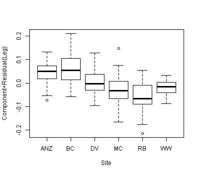
These are Component+Residual (Partial Residual) Plots

a component+residual plot

$\endgroup$
2
  • $\begingroup$ Thanks @BenBarnes, from this I can see that site RB has an intercept pretty low compared to BC. Is it the case that this comparison does not have to be significantly different in order for the model that fits each of these intercepts to be significantly better than the one that fits a single intercept? $\endgroup$ Commented Apr 17, 2012 at 17:35
  • $\begingroup$ @James, the anova() comparing lm.1 with lm.2 performs an F-test (en.wikipedia.org/wiki/F-test#Regression_problems), which basically compares the reduction in the residual sum of squares between two nested models to the residual sum of squares of the model with more terms. Therefore, it does not specifically take into consideration whether individual regression coefficients are statistically significant. Like @Manoel, I find Andrew Gelman's papers and books very helpful, especially "Data Analysis Using Regression and Hierarchical Models". $\endgroup$
    – BenBarnes
    Commented Apr 17, 2012 at 20:04
3
$\begingroup$

I think, among other things, that you're computing the confidence intervals wrong. Here are two ways to look at it:

(1) differences of each site from the baseline (ANZ) site [you could also compute differences from the overall mean by changing to sum-to-zero-contrasts

library(coefplot2)  ## on r-forge
coefplot2(lm.2)

or (2) all pairwise comparisons (I'm not fond of this approach, but it's common):

library(multcomp)
ci <- confint(glht(lm.2, linfct = mcp(Site = "Tukey")))
ggplot(fortify(ci),aes(lhs,estimate,ymin=lwr,ymax=upr))+
    geom_pointrange()+theme_bw()+geom_hline(yintercept=0,col="red")
$\endgroup$
1
  • $\begingroup$ The multcomp package approach gave this error: Error in as.data.frame.default(x[[i]], optional = TRUE, stringsAsFactors = stringsAsFactors) : cannot coerce class 'c("confint.glht", "glht")' into a data.frame $\endgroup$ Commented Apr 17, 2012 at 17:32
2
$\begingroup$

In addition to the other answers, here are some links from the Cornell Statistical Consulting Unit that are relevant to overlapping confidence intervals and serve as a good, short reminder of what they do and don't mean

http://www.cscu.cornell.edu/news/statnews/stnews73.pdf http://www.cscu.cornell.edu/news/statnews/Stnews73insert.pdf

Here's the main point:

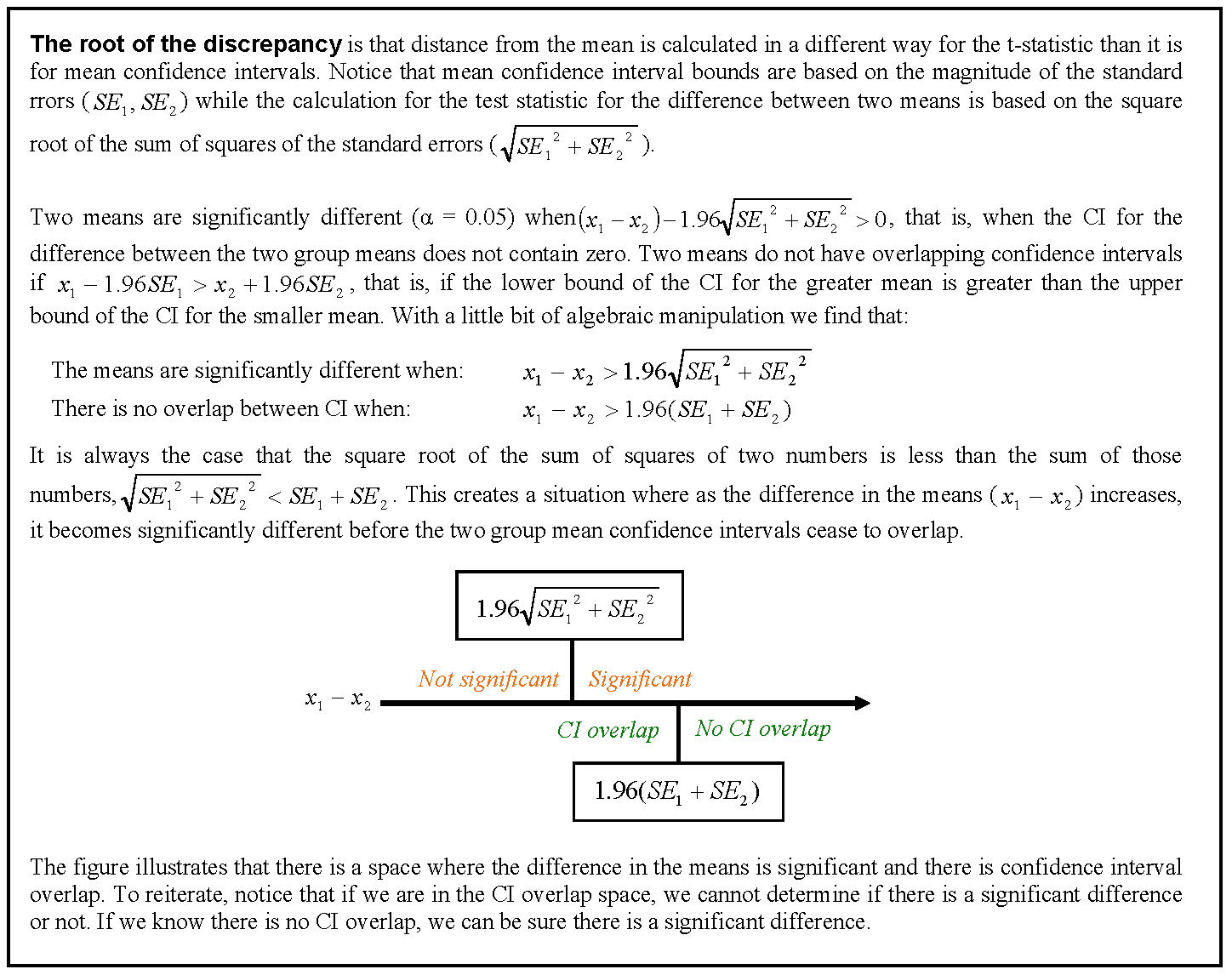
If two statistics have non-overlapping confidence intervals, they are necessarily significantly different but if they have overlapping confidence intervals, it is not necessarily true that they are not significantly different.

Here's the relevant text from the first link:

We can illustrate this with a simple example. Suppose we are interested in comparing means from two independent samples. The mean of the first sample is 9 and the mean of the second sample is 17. Let’s assume that the two group means have the same standard errors, equal to 2.5. The 95 percent confidence interval for the first group mean can be calculated as: ± × 5.296.19 where 1.96 is the critical t-value. The confidence interval for the first group mean is thus (4.1, 13.9). Similarly for the second group, the confidence interval for the mean is (12.1, 21.9). Notice that the two intervals overlap. However, the t-statistic for comparing two means is:

t = (17-9)/√(2.5² + 2.5²) = 2.26

which reflects that the null hypothesis, that the means of the two groups are the same, should be rejected at the α = 0.05 level. To verify the above conclusion, consider the 95 percent confidence interval for the difference between the two group means: (17-9)±1.96 x √(2.5² + 2.5²) which yields (1.09, 14.91). The interval does not contain zero, hence we reject the null hypothesis that the group means are the same.

Generally, when comparing two parameter estimates, it is always true that if the confidence intervals do not overlap, then the statistics will be statistically significantly different. However, the converse is not true. That is, it is erroneous to determine the statistical significance of the difference between two statistics based on overlapping confidence intervals. For an explanation of why this is true for the case of two-sample comparison of means, see the following link: http://www.cscu.cornell.edu/news/statnews/Stnews73insert.pdf

Here's the info from the other link:

enter image description here

$\endgroup$
1
$\begingroup$

Note that all your Head values are in the 1.7 - 2.4 range, while the intercepts are trying to estimate the Leg value at Head=0. This is a major extrapolation, so there is lots of uncertainty. If you were to center the Head values, and repeat this analysis, the confidence intervals would get much tighter.

Additionally, overlapping 95% confidence intervals do not imply lack of statistically significant difference. In fact, for two groups, non-overlapping 84% confidence intervals approximate having differences significant at the 5% level. Of course, because of multiple testing, this does not quite work with multiple groups.

$\endgroup$

Your Answer

By clicking “Post Your Answer”, you agree to our terms of service and acknowledge you have read our privacy policy.

Not the answer you're looking for? Browse other questions tagged or ask your own question.