Examples of connected designs in DOE

Question

I want to understand connectedness in block designs , I know this about connectedness: a design is said to be disconnected if we are able to create two separate groups (of blocks) such that they do not contain any common treatment (or any block in one group does not contain any treatment from other group), otherwise its called connected.

I just want to confirm the concept for more confidence with these two examples, please tell if my logic is wrong

example 1: consider the following design with 8 treatment and 4 blocks (fig 1):

example 2:again consider the following design with 8 treatment and 4 blocks (fig 2):

In fact there is no possible separation such that two groups will have no common treatment.

Answer 1

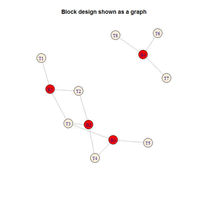
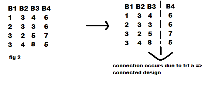
We can draw the block design as a graph, in the meaning of graph theory. I used the igraph package in R to draw: (this is your first example)

In this graph, the red vertices represents the blocks, and the antiquewhite vertices represents treatments. Edges are drawn between a block and a treatment if that treatment belongs to that block. The design is now connected if this graph is connected in the graph theory sense, that is, each pair of vertices is connected with some sequence of edges. We can see at once that this graph is not connected, in fact, we can see that it consists of two connected components. It follows that the design is not connected. (This is an example of a bipartite graph) (For some reason, the layout of the graph differs between calls to plot, in this case a second call would have given a better layout!)

To the Ops question, is my logic correct? yes, it is, and the figure above helps understand it.

Below is the R code I used to construct the plot. (It would maybe be useful to package this in R?)

library(ibd)
d1  <-  matrix(c(1, 2, 3, 3, 3, 3, 2, 4, 4, 3, 5, 5, 6, 6, 7, 8), 4, 
                 4, byrow=TRUE)
N1  <-  design_to_N(d1)
colnames(N1) <- c("B1", "B2", "B3", "B4")
rownames(N1)  <-  c("T1", "T2", "T3", "T4", "T5", "T6", "T7", "T8")
names(dimnames(N1))  <-  c("treatments", "blocks")
    
library(igraph)
    
G1  <-  graph_from_incidence_matrix(N1)
vertex_attr(G1) <-  list(color=c(rep("antiquewhite1", 8), rep("red", 
           4)),  names=c("T1", "T2", "T3", "T4", "T5", "T6", "T7", 
           "T8", "B1", "B2", "B3", "B4"))
plot(G1)
title("Block design shown as a graph")

The package ibd we used does have some other interesting functions and ideas, among them a function is.connected, but unfortunately it does seem to give the wrong answer on this example.

To connect all of this with the formal definition of a "connected design": A block design is connected if all elementary treatment contrasts has unbiased estimators. An interesting link where this definition is discussed is arXiv. Let the treatment effects be $\tau_1, \dotsc,\tau_8$, the block effects be $\beta_1, \dotsc, \beta_4$.

We can write a linear model for the design as $$ y_i = \mu + \beta_{b(i)} + \tau_{t(i)} +\epsilon_i, \qquad i=1, \dotsc, 16 $$ where $b(i)$ is the block corresponding to $i$ and $t(i)$ is the treatment corresponding to $i$. Then elementary treatment contrasts are estimators of the difference $\tau_j - \tau_{j'}$ for treatments $j \not= j'$.

It is possible to see that this can be done for a pair of treatment effects, if the corresponding vertices in the graph can be united in a chain of vertices, alternating white and red vertices which are united by an edge. For example, for $\tau_1, \tau_5$ such a chain is T1---B1---T2---B2---T4---B3---T5. You can construct another chain as an exercise. For $\tau_1, \tau_7$ no such chain exist, as can be easily seen from the graph.