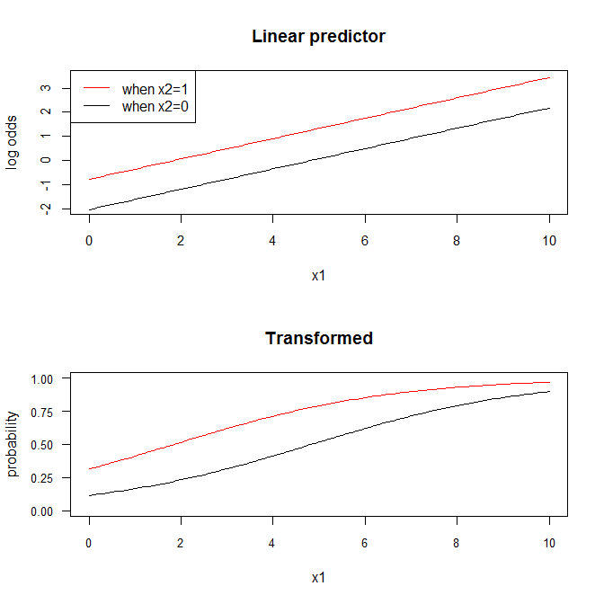
This is mostly addressed at What does “all else equal” mean in multiple regression? Namely, that they can be held constant at any value or level of the covariates. In some sense, it is easiest to explain them (or conceive of them) as being held at the means of the other continuous variables and the reference levels of the other categorical variables, but any value or level could be used. Furthermore, this assumes that there are no interaction terms in the model amongst your covariates, otherwise it is not generally possible to hold all else equal (that is also explained in the linked thread).
The only added complication in a logistic regression context (or any generalized linear model in which the link is not the identity function), is that this only pertains to the linear predictor. For example, in logistic regression, the result of $\bf X \boldsymbol{\hat\beta}$ is a set of log odds. However, people often prefer to see $\hat p_i$, instead. That is of course fine, but it involves a nonlinear transformation. As a result, due to Jensen's inequality, the sigmoid curves you would get for the relationship between $X_1$ and $Y$ would differ based on whether $X_2$ is held constant at $\bar X_2$ or $\bar X_2 + s_{\bar X_2}$. The implication of this is that there isn't really any such thing as "all else equal" in the transformed space, only in the space of the linear predictor.
If it helps to clarify these ideas, consider this simple simulation (coded in R):
set.seed(6666)                              # makes the example exactly reproducible
lo2p = function(lo){ exp(lo)/(1+exp(lo)) }  # we'll need this function

x1 = runif(500, min=0, max=10)     # generating X data
x2 = rbinom(500, size=1, prob=.5)
lo = -2.2 + 1.1*x2 + .44*x1        # the true data generating process
p  = lo2p(lo)
y  = rbinom(500, size=1, prob=p)   # generating Y data

m  = glm(y~x1+x2, family=binomial) # fitting the model & viewing the coefficients
summary(m)$coefficients
#               Estimate Std. Error   z value     Pr(>|z|)
# (Intercept) -2.0395304 0.25907518 -7.872350 3.480415e-15
# x1           0.4220811 0.04409752  9.571538 1.053267e-21
# x2           1.2582332 0.22653761  5.554191 2.789001e-08

x.seq   = seq(from=0, to=10, by=.1)  # this is a sequence of X values for the plot
x2.0.lo = predict(m, newdata=data.frame(x1=x.seq, x2=0), type="link") # predicted
x2.1.lo = predict(m, newdata=data.frame(x1=x.seq, x2=1), type="link") # log odds
x2.0.p  = lo2p(x2.0.lo)  # converted to probabilities
x2.1.p  = lo2p(x2.1.lo)

windows()
  layout(matrix(1:2, nrow=2))
  plot(x.seq,  x2.0.lo, type="l", ylim=c(-2,3.5), ylab="log odds", xlab="x1",
       cex.axis=.9, main="Linear predictor")
  lines(x.seq, x2.1.lo, col="red")
  legend("topleft", legend=c("when x2=1", "when x2=0"), lty=1, col=2:1)

  plot(x.seq,  x2.0.p, type="l", ylim=c(0,1), yaxp=c(0,1,4), cex.axis=.8, las=1,
       xlab="x1", ylab="probability", main="Transformed")
  lines(x.seq, x2.1.p, col="red")

On the scale of the linear predictor (i.e., the log odds), the slope on $X_1$ is $\approx 1.26$ whether you are holding $X_2$ at $0$ or $1$. That's because the lines are parallel. On the other hand, in the transformed space, the lines aren't parallel. The rate of change in $\hat p(Y=1)$ associated with a $1$-unit change in $X_1$ differs depending on whether $X_2 = 0$ or $X_2 = 1$. (It also differs depending on what value of $X-1$ you are starting from.)

