How to use blasso function in R package "monomvn"? [closed]

Question

I am a freshman with Bayesian lasso. I searched online and found that the only package I can use is monomvn. There's only one example about diabetes data in its R document. However, the parameters set in that example is quietly simply. Just "blasso(x,y)". I tried to follow this but when it comes to my data, all coefficients were shrunk to zeros. Should I give initial values to beta? Appreciate it if anyone could provide examples describing how to set parameters for this function? Thanks a lot.

Answer 1

I am not an expert but I would be happy to share my experience with the monomvn package.

Should I give initial values to beta?

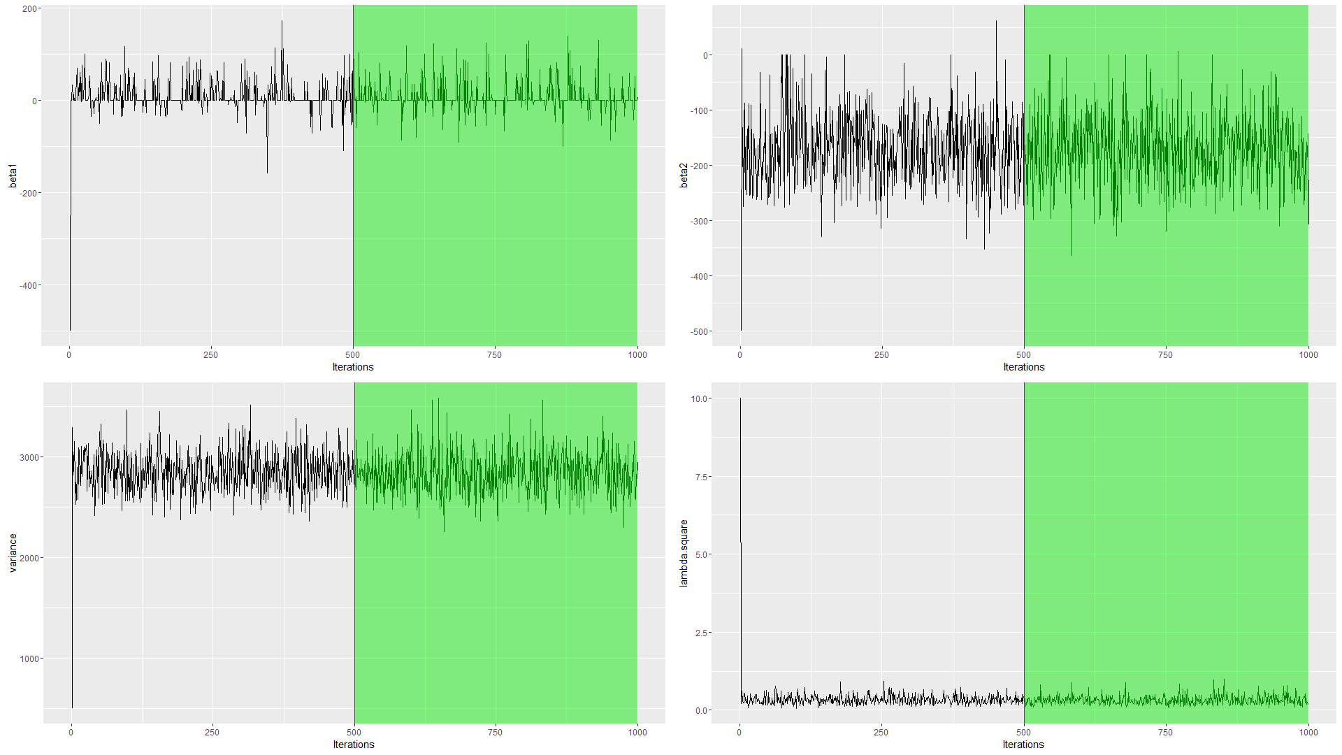
Given enough iterations, initial values shouldn't have any impact on any parameter (e.g. regression coefficients, error variance and penalty parameter). Please consider the R code and traceplots below:

# load required packages and datasets
library(monomvn); library(lars); library(glmnet); library(miscTools) 
data(diabetes); attach(diabetes)

# define the burn-in period, number of mcmc samples to be drawn and initial values 
burnin <- 500
iter <- 1000
initial.beta <- rep(-500, dim(x2)[2]) # assigning an extreme initial value for all betas
initial.lambda2 <- 10 # assigning an extreme initial value for lambda (penalty parameter)
initial.variance <- 500 # assigning an extreme initial value for variance parameter

# starting the Gibbs sampler here
lasso <- blasso(X = x2, # covariate matrix with dimensions 442 x 64
                y = y,  # response vector with length of 442
                T = iter, # number of iterations
                beta = initial.beta, 
                lambda2 = initial.lambda2,  
                s2 = initial.variance)

# collecting draws for some of the parameters for visualization
coef.lasso <- as.data.frame(cbind(iter = seq(iter), 
                              beta1 = lasso$beta[, "b.1"], 
                              beta2 = lasso$beta[, "b.2"], 
                              variance = lasso$s2, 
                              lambda.square = lasso$lambda2))

To get the parameter estimations, I would use the posterior median as Park and Casella (2008) have done.

> colMedians(coef.lasso[-seq(burnin), -1])
beta1       beta2        variance         lambda.square 
0.0000000  -172.3840906  2841.4410472     0.3031814 

Please consider that I have computed the coefficients after discarding first half of the draws. Since I have considered only the draws from green-shaded areas, those extreme initial values I have assigned above have no impact on the posterior medians anymore.

I tried to follow this but when it comes to my data, all coefficients were shrunk to zeros.

Let's now compare lasso (glmnet package) and Bayesian lasso (monomvn package)

fit.glmnet <-  glmnet(as.matrix(x2), y, 
                        lambda=cv.glmnet(as.matrix(x2), y)$lambda.1se)
coef.glmnet <- coef(fit.glmnet)
sum(coef.glmnet == 0)
53

The original lasso implementation has shrunk 53 parameters to 0. Let's now check Bayesian lasso:

sum(colMedians(lasso$beta[-seq(burnin), ]) == 0)
56

and it shrank 56 out of 64 exactly to 0.

Please also note that your estimation results might significantly differ when you specify the prior distributions. A quick example would be to change the parameters using the 'rd' argument in blasso() where 'rd' controls the gamma prior on lambda^2. (please hit ?blasso for other hyperprior specifications)

Here is an example:

lasso2 <- blasso(X = x2, # covariate matrix with dimensions 442 x 64
                 y = y,  # response vector with length of 442
                 T = iter, # number of iterations
                 beta = initial.beta, 
                 lambda2 = initial.lambda2,  
                 s2 = initial.variance,
                 rd = c(1, 1.78)) # hyperparameters suggested by Park & Casella (2008)

coef.lasso2 <- as.data.frame(cbind(iter = seq(iter), 
                                  beta1 = lasso2$beta[, "b.1"], 
                                  beta2 = lasso2$beta[, "b.2"], 
                                  variance = lasso2$s2, lambda.square = 
                                  lasso$lambda2))

 colMedians(coef.lasso2[-seq(burnin), -1]) # new posterior median estimations
 beta1         beta2        variance         lambda.square 
 0.0000000    -183.7851178  2817.3811240     0.2313924 

I hope it is now clear now that giving initial values doesn't really help. Have you tried estimating the parameters using glmnet? If the results differ a lot, then you might consider tuning the hyperpriors on parameters in blasso(). If you still get the same results, maybe the parameters are all indeed 0 :-)

Hope that helps!