Nothing will be able to prove it one way or another, because even if you find revenue has dropped from that time, you will not be able to dismiss the possibility of other structural change (eg new competitor, changed regulatory environment, changed fashion, something you can't even think of...).
You can use time series techniques to identify if the timing of the changed system is associated with a decline in revenue; or, better for your aims, you might be able to dismiss that claim (and if there's no obvious decline, there's nothing to explain, right? well, maybe... the problem is constructing a counterfactual.).
Problems you will have to deal with will include; seasonality (both micro eg weekly and macro eg summer v winter); growth or other trends; and serial correlation of your observations.
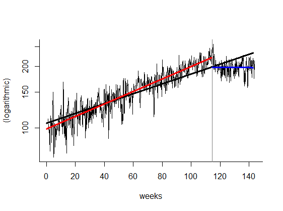
In the plot below from simulated data you can see one way of going about this.
You can fit a model of some sort based on there being no change over time - in this case, I've fit a linear model with the response variable on a logarithmic scale, which is equivalent to saying the daily revenue is growing at a constant rate. This null hypothesis is shown with the black line.
The red and blue lines, on the other hand, show an alternative, more complex model, which allows both a change in the level of revenue and a change in the growth rate (in this case to negative) as a result of the introduction of the new system. Once you've fit this more complex model as well, you can then test for statistically significant evidence that this model is needed rather than the simple black line model.

(Note that in this case, if you did a simple t test comparing before and after situations as @pgericson suggests, you'd conclude you'd significantly increased revenue with the new system, because of the underlying growth rate in the months leading up to the new system.)
Now, the danger to look out for, is you can't just fit a model in the way you would with cross sectional data. You need to allow for the fact that a revenue observation one day does not add that much to the revenue observation the day before - they are probably highly correlated and not completely new information. Any stats or econometric package worth its salt will allow this; in R you can use either gls() in the nlme library or arima() to do it.
My R code that simulated this data and did some basic analysis on it is pasted below.
#simulate data
set.seed(80)
x <- ts(100*exp(1:1000*0.001), frequency=7)
e <- rnorm(1002,0,10)
x <- x+ 0.5*e[1:1000] + 0.8*e[2:1001] + e[3:1002]
changed <- rep(c(0,1), c(800,200))
x <- x + cumsum(changed)^0.4 * rnorm(1000, -8,1)

# check it looks ok
par(mfrow=c(2,1))
plot(x, main="Daily revenue ($'000)", xlab="weeks", ylab="(original)")
abline(v=801/7, col="grey50")
plot(x, ylab="(logarithmic)", xlab="weeks", log="y")
abline(v=801/7, col="grey50")


# t test makes it look like you've increased revenue! -
# because it ignores the trend
t.test(x~changed)

# Much better is to illustrate in some kind of model
# that can take into account any growth trend.
# With real data this will be quite complex, but
# in my simulated data the growth is nice and regular
# so it is easy to see if it is disrupted.

x.df <- data.frame(x=x, changed=changed, day=1:1000)
win.graph()
x.lm1 <- lm(log(x)~day, data=x.df)
plot(x, ylab="(logarithmic)", xlab="weeks", log="y", bty="l")
abline(v=801/7, col="grey50")
lines(1:1000/7, exp(predict(x.lm1)), lwd=3)

x.lm2 <- lm(log(x)~day*changed, data=x.df)
lines(1:800/7, exp(predict(x.lm2))[1:800], col="red", lwd=3)
lines(801:1000/7, exp(predict(x.lm2))[801:1000], col="blue", lwd=3)
anova(x.lm2) # shows "changed" is significant
summary(x.lm2) # could be used to estimate how much change has happened


# The problem with this approach though is that
# the errors are serially correlated and hence the inferences
# based on them being iid will not be justifiable.  As shown by this diagnostic
# plot:
acf(residuals(x.lm2))


library(nlme)
x.lm3 <- gls(log(x)~day*changed, data=x.df, correlation=corAR1())
anova(x.lm3) # "changed" is still significant but much higher p values
summary(x.lm3)

# I'd like to fit a model with more lags in the autoregression structure
# but the following code takes frigging ages for some reason (eventually came out OK)
x.lm4 <- update(x.lm3, correlation=corARMA(c(0.6, 0.2), p=2, q=0),
    control=glsControl(msVerbose=TRUE))

