20
$\begingroup$

I have two time-series:

  1. A proxy for the market risk premium (ERP; red line)
  2. The risk-free rate, proxied by a government bond (blue line)
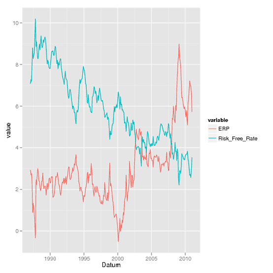
Risk premium proxy and risk-free rate over time

I want to test if the risk-free rate can explain the ERP. Hereby, I basically followed the advice of Tsay (2010, 3rd edition, p. 96): Financial Time Series:

  1. Fit the linear regression model and check serial correlations of the residuals.
  2. If the residual series is unit-root nonstationarity, take the first difference of both the dependent and explanatory variables.

Doing the first step, I get the following results:

Coefficients:
               Estimate Std. Error t value Pr(>|t|)    
(Intercept)     6.77019    0.25103   26.97   <2e-16 ***
Risk_Free_Rate -0.65320    0.04123  -15.84   <2e-16 ***
---
Signif. codes:  0 ‘***’ 0.001 ‘**’ 0.01 ‘*’ 0.05 ‘.’ 0.1 ‘ ’ 1 

As expected from the figure, the relation is negative and significant. However, the residuals are serially correlated:
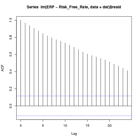
ACF function of the residuals of the regression of risk-free rate on ERP

Therefore, I first difference both the dependent and explanatory variable. Here is what I get:

Coefficients:
                Estimate Std. Error t value Pr(>|t|)    
(Intercept)    -0.002077   0.016497  -0.126      0.9    
Risk_Free_Rate -0.958267   0.053731 -17.834   <2e-16 ***
---
Signif. codes:  0 ‘***’ 0.001 ‘**’ 0.01 ‘*’ 0.05 ‘.’ 0.1 ‘ ’ 1

And the ACF of the residuals looks like:
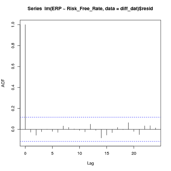
ACF function of the residuals of the regression of risk-free rate on ERP (differenced)

This result looks great: First, the residuals are now uncorrelated. Second, the relation seems to be more negative now.

Here are my questions (you probably wondered by now ;-) The first regression, I would have interpreted as (econometric problems aside) "if the riskfree rate rises by one percentage point, the ERP falls by 0.65 percentage points." Actually, after pondering about this for a while, I would interpret the second regression just the same (now resulting in a 0.96 percentage points fall though). Is this interpretation correct? It just feels weird that I transform my variables, but don't have to change my interpretation. If this, however, is correct, why do the results change? Is this just the result of econometric problems? If so, does anyone have an idea why my second regression seems to be even "better"? Normally, I always read that you can have spurious correlations that vanish after you do it correctly. Here, it seems the other way round.

$\endgroup$

2 Answers 2

28
$\begingroup$

Suppose that we have the model $$\begin{equation*} y_t = \beta_0 + \beta_1 x_t + \beta_2 t + \epsilon_t. \end{equation*}$$ You say that these coefficients are easier to interpret. Let's subtract $y_{t-1}$ from the lefthand side and $\beta_0 + \beta_1 x_{t-1} + \beta_2 ({t-1}) + \epsilon_{t-1}$, which equals $y_{t-1}$, from the righthand side. We have $$\begin{equation*} \Delta y_t = \beta_1 \Delta x_t + \beta_2 + \Delta \epsilon_t. \end{equation*}$$ The intercept in the difference equation is the time trend. And the coefficient on $\Delta x$ has the same interpretation as $\beta_1$ in the original model.

If the errors were non-stationary such that $$\begin{equation*} \epsilon_t = \sum_{s=0}^{t-1}{\nu_s}, \end{equation*}$$ such that $\nu_s$ is white noise, the the differenced error is white noise.

If the errors have a stationary AR(p) distribution, say, then the differenced error term would have a more complicated distribution and, notably, would retain serial correlation. Or if the original $\epsilon$ are already white noise (An AR(1) with a correlation coefficient of 0 if you like), then differencing induces serial correlation between the errors.

For these reasons, it is important to only difference processes that are non-stationary due to unit roots and use detrending for so-called trend stationary ones.

(A unit root causes the variance of a series to change and it actually explode over time; the expected value of this series is constant, however. A trend stationary process has the opposite properties.)

$\endgroup$
10
  • $\begingroup$ Great answer, thanks for the explanation. That helps a lot. $\endgroup$ Commented May 3, 2012 at 21:41
  • 3
    $\begingroup$ +1 The last sentence is gold, and I wish I'd seen it stated so clearly when I first encountered the idea of differencing. $\endgroup$
    – Wayne
    Commented May 3, 2012 at 23:24
  • $\begingroup$ Charlie, would you mind adding some clarifications of a couple of things? First you say that "if the $\epsilon$ are white noise, then so too is the difference". What do you mean by this? If I take the difference of a white-noise process, the result is pretty strongly autocorrelated! Also, what do you mean by "detrending" a stationary time series? This sounds contradictory to me in the sense that a stationary time series, by definition, has no trend. Maybe in the latter case you're referring only to the noise structure and not the series itself(?). Cheers. $\endgroup$
    – cardinal
    Commented May 4, 2012 at 0:12
  • 1
    $\begingroup$ @Christoph_J, You have that $y$ today is correlated with $y$ yesterday; your ACF shows that. The $x$ today is likely correlated with $x$ yesterday. The $x$ yesterday is correlated with the $y$ yesterday. As such, the included predictor $x$ is correlated with an omitted variable $y_{t-1}$ and you have an omitted variables bias issue. Differencing breaks those correlations and averts the omitted variables problem. $\endgroup$
    – Charlie
    Commented May 4, 2012 at 15:22
  • 1
    $\begingroup$ @Charlie can I understand your response to suggest that the interpretation of the $\beta_{i}$ where i>0 is the same as if you never differenced? Here was my question on this site and I would love to get an expert opinion. Thanks! stats.stackexchange.com/questions/169838/… $\endgroup$
    – B_Miner
    Commented Sep 9, 2015 at 15:05
2
$\begingroup$

First differencing removes linear trends that seem to persist in your original residuals. It looks like the first differencing removed the trend in the residuals and you are left with basically uncorrelated residuals. I am thinking that maybe the trend in the residuals hid part of the negative relationship between ERP and risk free rate and that would be the reason why the model shows a stronger relationship after differencing.

$\endgroup$
0

Your Answer

By clicking “Post Your Answer”, you agree to our terms of service and acknowledge you have read our privacy policy.

Not the answer you're looking for? Browse other questions tagged or ask your own question.