An answer partly depends on what you mean by the word "test" there.
If you're after a formal hypothesis test, one could try to perform some test based on the likelihood or the log of the likelihood (as per Fisher) or if there's a specific alternative via a likelihood ratio test, though various tests might be devised depending on broader classes of alternatives that should perform pretty well.
My advice would not be to pursue formal tests of goodness of fit. Our models are (usually) just that -- models, not perfect descriptions. As such in large samples they're clearly wrong (even though the model may be a very good description of the thing we're modelling) and in small samples the fact that we can't clearly tell these models are wrong should be no consolation, since in a small sample even a quite poor model may be hard to clearly identify. A clearly wrong model - one we would reject via a test - may remain highly useful, if the deviation from correctness has small effects on our inference (i.e. we're dealing more with raw-effect-size type problems rather than statistical significance)
As such I'd tend to lean toward diagnostic displays rather than formal tests, though if you can be much more specific about what effects will matter, there may be some uses for testing.
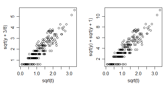
One approach to displays would be to check the mean-variance relationship. In particular, if we let $Y_i$ be the $i$-th increment in count and we let $s_i$ be the corresponding increment in time, then under the Poisson assumption $Y_i\sim \text{Pois}(\lambda s_i)$. If it's Poisson the mean should be proportional to $s_i$ and the variance should be proportional to $s_i$ (or standard deviation proportional to $\sqrt{s_i}$).
This is easier to see on the square root scale. If the Poisson means are not typically very small (so the observations aren't nearly all 0 or 1) you can plot either $\sqrt{y_i+\frac38}$ or $\sqrt{y_i}+\sqrt{y_i+1}$ against $\sqrt{s_i}$ -- either one should look approximately linear with fairly constant spread:

The first transformation in the Anscombe transformation for the Poisson, the second is the Freeman-Tukey transformation.
It's possible to adjust the $\sqrt{s_i}$ for each plot to be closer to the expected value of the transformed $Y$ for small $\lambda s_i$ which can improve the appearance of the plot a bit when the mean is smaller, but it's usually not necessary.
There are other options that can work as well.
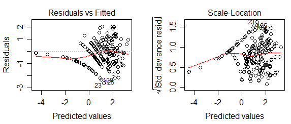
You might even consider an examination of a suitable choice of residuals vs fitted and a scale vs fitted from a constant-only Poisson glm fit with log link and an offset of $\log(s_i)$, but these can be considerably harder to interpret. This is one where the model is correct (the same data as above):

(Personally I find the earlier plots easier to judge)


