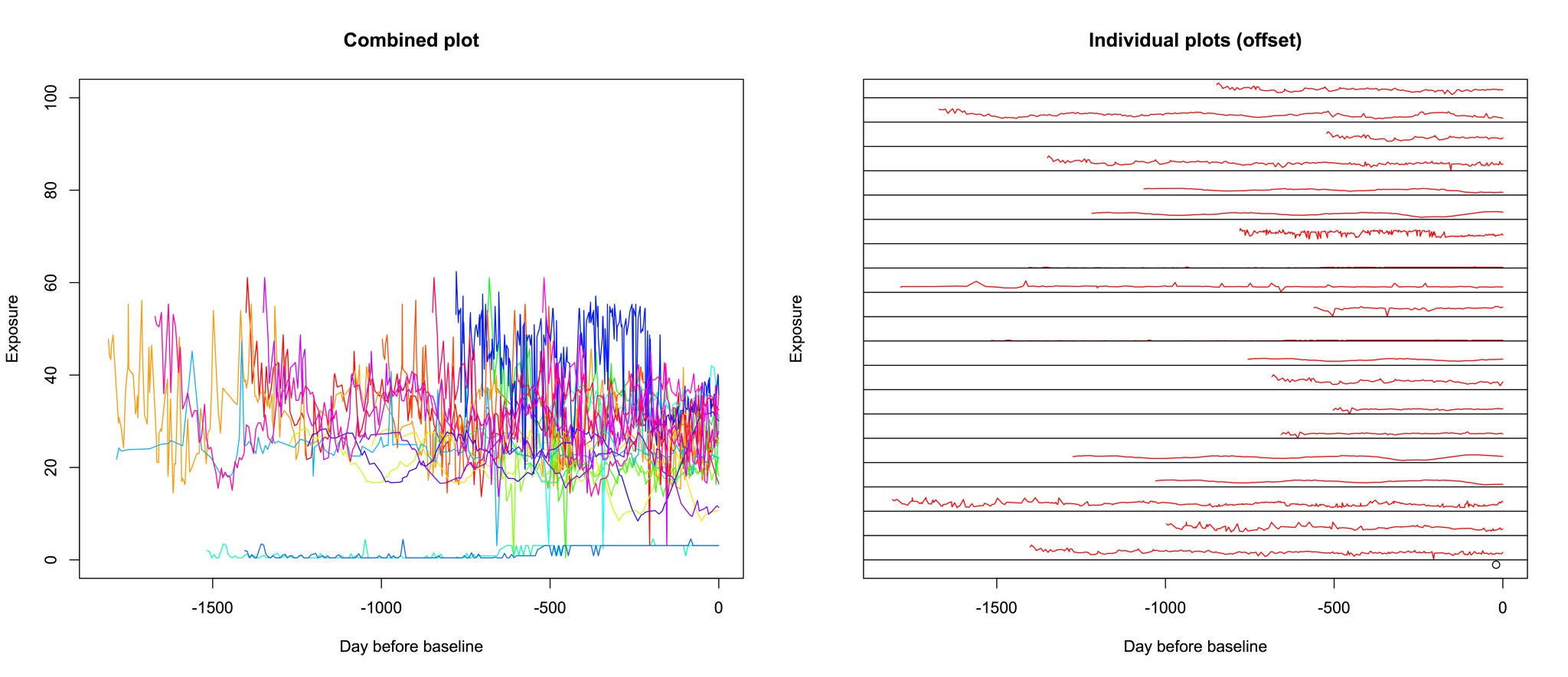
An interesting question. The main issue here is that the lack of a blood pressure measurement at the start of the experiment introduces a confounding effect: anyway, the large number of participants and the fact that other covariates are measured, which correlate with blood pressure, may help mitigate the issue.
What I would do, would be first of all to perform a purely cross-sectional study, where you substitute the history of exposure by some summary of it (for example, the time-averaged exposure), and see if controlling for all other covariates this shows an effect on BP. In doing this you are of course throwing away information, but it can at least give you an idea of what's happening.
Secondly, you could try to fit a linear scalar-on-function regression model (see also here for a freely downloadable copy):
$$y_i=\alpha_0+\boldsymbol{\alpha}^T\mathbf{x}_i+\int_0^T\beta(s)\mathcal{X}_i(s)\text{d}s+\epsilon_i, \qquad i=1,\dots,N$$
Some explanations are in order here:
$\alpha_0$ is the intercept, and $\boldsymbol{\alpha}$ is the vector
of coefficients for the scalar covariates $\mathbf{x}_i$, i.e., age,
physical activity, smoking, social class, etc.
$\mathcal{X}_i(t)$ is a "functional covariate", i.e., it's simply a real function of time on the interval $I=[0,T]$. In your case, i's the time series of the exposure
- $\beta(t)$ is called a coefficient function, and like $\alpha_0$ and $\boldsymbol{\alpha}$, it must be estimated
- finally, $\epsilon_i$ are iid, mean 0, constant variance errors, usually assumed to be normally distributed
The model can be extended by including random effects, and this would surely be useful in your case, because certainly there will be some subject-specific effects (two different persons won't exhibit the same response to the same history of exposure). However, I don't see how you could estimate them, given that you have just one functional covariate for subject; it's not like you repeated the five years exposure experiment, multiple times for a same subject.
There are basically two different ways to estimate such a model: one is a fixed-basis approach, where the coefficient function is expanded in a data-independent basis of functions (usually splines):
$$\beta(t)=\mathbf{b}(t)^T\boldsymbol{\gamma}$$
where $\mathbf{b}(t)=[b_1(t),\dots,b_K(t)]$ is the set of basis functions and $\boldsymbol{\gamma}=(\gamma_1,\dots,\gamma_K)$ are the coefficients of $\beta(t)$ in the basis $\mathbf{b}(t)$. Then, we find the coefficients $(\alpha_0,\boldsymbol{\alpha},\boldsymbol{\gamma})$ which minimize the sum of squared differences between the response and the model, plus a penalty to prevent overfitting.
The other approach uses a data-driven basis, usually the eigenfunction of the covariance function $Cov[\mathcal{X}_i(t),\mathcal{X}_i(s)]$. This approach might be more suitable in your case since your time series are irregularly sampled.
Once you have fit the model, you may be interested in testing the hypothesis that the coefficient function is zero as opposed to it being non-zero for some time instant, or the hypothesis that the coefficient function is constant, etc.
R packages that implement scalar-on-function regression as well as various hypothesis tests are mgcv and refund, for example.
The only issue I see with this framework, as applied to your problem, is that instead of having all your functional covariates defined on the same time interval $I=[0,T]$, you actually have a random time interval $I_i=[t_i,T]$ for each subject. I have no idea how to deal with that: a multilevel model where $t_i$ has some prior distribution, and $y|t_i$ is modelled with the linear scalar-on-function regression model above, might work. I've never seen it used, though. Maybe you could ask another question, specifically on how to model the random initial time....

