Is the Error rate a Convex function of the Regularization parameter lambda?

Question

In choosing the regularization parameter lambda in Ridge or Lasso the recommended method is to try different values of lambda, measure the error in the Validation Set and finally chose that value of lambda that returns the lowest error.

It is not cleat to me if the function f(lambda) = error is Convex. Could it be like this? I.e. could this curve have more than one local minima (which would imply that finding a minimum of the Error at some region of lambda does not preclude the possibility that in some other region there is a lambda returning an even smaller Error)

Your advice will be appreciated.

Answer 1

The original question asked whether the error function needs to be convex. No, it does not. The analysis presented below is intended to provide some insight and intuition about this and the modified question, which asks whether the error function could have multiple local minima.

Intuitively, there doesn't have to be any mathematically necessary relationship between the data and the training set. We should be able to find training data for which the model initially is poor, gets better with some regularization, and then gets worse again. The error curve cannot be convex in that case--at least not if we make the regularization parameter vary from $0$ to $\infty$.

Note that convex is not equivalent to having a unique minimum! However, similar ideas suggest multiple local minima are possible: during regularization, first the fitted model might get better for some training data while not appreciably changing for other training data, and then later it will get better for other training data, etc. A suitable mix of such training data ought to produce multiple local minima. To keep the analysis simple I won't attempt to show that.

Edit (to respond to the changed question)

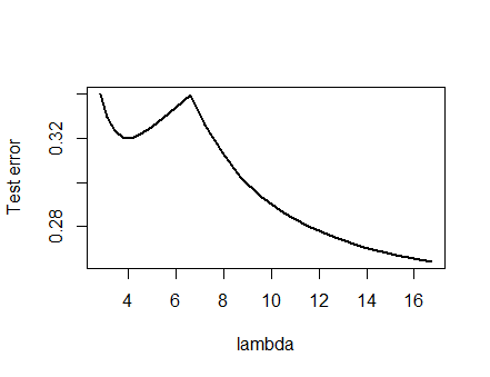
I was so confident in the analysis presented below and the intuition behind it that I set about finding an example in the crudest possible way: I generated small random datasets, ran a Lasso on them, computed the total squared error for a small training set, and plotted its error curve. A few attempts produced one with two minima, which I will describe. The vectors are in the form $(x_1,x_2,y)$ for features $x_1$ and $x_2$ and response $y$.

Training data

$$(1,1,-0.1),\ (2,1,0.8),\ (1,2,1.2),\ (2,2,0.9)$$

Test data

$$(1,1,0.2),\ (1,2,0.4)$$

The Lasso was run using glmnet::glmmet in R, with all arguments left at their defaults. The values of $\lambda$ on the x axis are the reciprocals of the values reported by that software (because it parameterizes its penalty with $1/\lambda$).

An error curve with multiple local minima

---

Analysis

Let's consider any regularization method of fitting parameters $\beta=(\beta_1, \ldots, \beta_p)$ to data $x_i$ and corresponding responses $y_i$ that has these properties common to Ridge Regression and Lasso:

1. (Parameterization) The method is parameterized by real numbers $\lambda \in [0, \infty)$, with the unregularized model corresponding to $\lambda=0$.

2. (Continuity) The parameter estimate $\hat\beta$ depends continuously on $\lambda$ and the predicted values for any features vary continuously with $\hat\beta$.

3. (Shrinkage) As $\lambda\to\infty$, $\hat\beta\to 0$.

4. (Finiteness) For any feature vector $x$, as $\hat\beta\to 0$, the prediction $\hat y(x) = f(x, \hat\beta) \to 0$.

5. (Monotonic error) The error function comparing any value $y$ to a predicted value $\hat y$, $\mathcal{L}(y, \hat y)$, increases with the discrepancy $|\hat y - y|$ so that, with some abuse of notation, we may express it as $\mathcal{L}(|\hat y - y|)$.

(Zero in $(4)$ could be replaced by any constant.)

Suppose the data are such that the initial (unregularized) parameter estimate $\hat\beta(0)$ is not zero. Let's construct a training data set consisting of one observation $(x_0, y_0)$ for which $f(x_0, \hat\beta(0))\ne 0$. (If it's not possible to find such an $x_0$, then the initial model won't be very interesting!) Set $y_0=f(x_0, \hat\beta(0))/2$.

The assumptions imply the error curve $e: \lambda \to \mathcal{L}(y_0, f(x_0, \hat\beta(\lambda))$ has these properties:

1. $e(0) = \mathcal{L}(y_0, f(x_0, \hat\beta(0)) = \mathcal{L}(y_0, 2y_0) = \mathcal{L}(|y_0|)$ (because of the choice of $y_0$).

2. $\lim_{\lambda\to\infty}e(\lambda) = \mathcal{L}(y_0, 0) = \mathcal{L}(|y_0|)$ (because as $\lambda\to\infty$, $\hat\beta(\lambda)\to 0$, whence $\hat{y}(x_0)\to 0$).

Thus, its graph continuously connects two equally high (and finite) endpoints.

Qualitatively, there are three possibilities:

• The prediction for the training set never changes. This is unlikely--just about any example you choose will not have this property.

• Some intermediate predictions for $0\lt \lambda \lt \infty$ are worse than at the start $\lambda=0$ or in the limit $\lambda\to\infty$. This function cannot be convex.

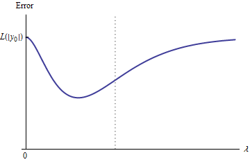
• All intermediate predictions lie between $0$ and $2y_0$. The continuity implies there will be at least one minimum of $e$, near which $e$ must be convex. But since $e(\lambda)$ approaches a finite constant asymptotically, it cannot be convex for large enough $\lambda$.

The vertical dashed line in the figure shows where the plot changes from convex (at its left) to non-convex (to the right). (There is also a region of non-convexity near $\lambda\approx 0$ in this figure, but this won't necessarily be the case in general.)

Answer 2

$\newcommand{\dbeta}{\frac{\partial}{\partial \lambda} \hat\beta_\lambda}$ $\newcommand{\ddbeta}{\frac{\partial^2}{{\partial \lambda}^2} \hat\beta_\lambda}$

This answer specifically concerns the lasso (and does not hold for ridge regression.)

Setup

Suppose that we have $p$ covariates that we're using to model a response. Suppose that we have $n$ training data points and $m$ validation data points.

Let the training input be $X_{(1)} \in \mathbb{R}^{n \times p}$ and response be $y_{(1)} \in \mathbb{R}^n$. We will use the lasso on this training data. That is, put $$\hat\beta_\lambda = \arg\min_{\beta \in \mathbb{R}^p} \|y_{(1)} - X_{(1)} \beta\|_2^2 + \lambda \|\beta\|_1, \tag{1}$$ a family of coefficients estimated from the training data. We will choose which $\hat\beta_\lambda$ to use as our estimator based on its error on a validation set, with input $X_{(2)} \in \mathbb{R}^{m \times p}$ and response $y_{(2)} \in \mathbb{R}^m$. With $$\hat\lambda = \arg\min_{\lambda \in \mathbb{R}_+} \|y_{(2)} - X_{(2)} \hat\beta_\lambda\|_2^2, \tag{2}$$ we are interested in studying the error function $e(\lambda) = \|y_{(2)} - X_{(2)} \hat\beta_\lambda\|_2^2$ which gives rise to our data-driven estimator $\hat\beta_{\hat\lambda}$.

Calculation

Now, we will calculate the second derivative of the objective in equation $(2)$, without making any distributional assumptions on the $X$'s or $y$'s. Using differentiation and some reorganization, we (formally) compute that \begin{align*} \frac{\partial^2}{{\partial \lambda}^2} \|y_{(2)} - X_{(2)} \hat\beta_\lambda\|_2^2 & = \frac{\partial}{\partial \lambda} \left\{ -2 y_{(2)}^T X_{(2)} \dbeta + 2 \hat\beta_\lambda^T X_{(2)}^T X_{(2)} \dbeta \right\} \\ & = -2 y_{(2)}^T X_{(2)} \ddbeta + 2 \left( \hat\beta_\lambda \right)^T X_{(2)}^T X_{(2)} \ddbeta + 2 \dbeta^T X_{(2)}^T X_{(2)}^T \dbeta \\ & = -2 \left\{ \left( y_{(2)} - X_{(2)} \hat\beta_\lambda \right)^T \ddbeta - \|X_{(2)} \dbeta\|_2^2 \right\}. \end{align*} Since $\hat\beta_\lambda$ is piecewise linear for $\lambda \not\in K$ (for $K$ being the finite set of knots in the lasso solution path), the derivative $\dbeta$ is piecewise constant and $\ddbeta$ is zero for all $\lambda \not\in K$. Therefore, $$\frac{\partial^2}{{\partial \lambda}^2} \|y_{(2)} - X_{(2)} \hat\beta_\lambda\|_2^2 = 2 \|X_{(2)} \dbeta\|_2^2,$$ a non-negative function of $\lambda$.

Conclusion

If we assume further that $X_{(2)}$ is drawn from some continuous distribution independent of $\{X_{(1)}, y_{(1)} \}$, the vector $X_{(2)} \dbeta \neq 0$ almost surely for $\lambda < \lambda_\max$. Therefore, the error function $e(\lambda)$ has second derivative on $\mathbb{R} \setminus K$ which is (almost surely) strictly positive. However, knowing that that $\hat\beta_\lambda$ is continuous, we know that the validation error $e(\lambda)$ is continuous.

Finally, from the lasso dual, we know that $\|X_{(1)} \hat\beta_\lambda\|_2^2$ decreases monotonically as $\lambda$ increases. If we can establish that $\|X_{(2)} \hat\beta_\lambda\|_2^2$ is also monotonic, then the strong convexity of $e(\lambda)$ follows. However, this holds with some probability approaching one if $\mathcal{L} \left( X_{(1)} \right) = \mathcal{L} \left( X_{(2)} \right)$. (I'll fill in details here soon.)