This is a fascinating question because (a) this issue does come up in practical work and (b) its solution can reveal hidden information in the data. Such is the case for the 80 values given in the post.
Most numbers represented in floating point format are far more precise than the data that originally produced them. No physical quantity, for instance, has ever been measured to more than 10 significant figures. Measurement systems vary widely. Analog instruments allow us to read numbers from graduated values marked on rulers or dials: these are inherently quantized to relatively low precision, usually only two or three significant figures (relative to some baseline). Other instruments may return rational numbers (with small denominators). Geiger counters and other radiological instruments, which count things and divide by some standard interval, are examples. Some digital instruments collect analog input but then round them to some power of two. Photosensors do something like this.
In many such cases, a set of numbers collected by an instrument may have a common denominator. That denominator might not be apparent in the decimal representations of the numbers. For instance, consider this set of random numbers between $0$ and $1$:
0.00947867298578199 0.23696682464454977 0.36966824644549762 0.41232227488151657
0.55924170616113744 0.60189573459715640 0.71563981042654023 0.86729857819905209
Although they certainly look random when represented as decimals, consider this representation of the original data:
2/211 50/211 78/211 87/211 118/211 127/211 151/211 183/211
Being integral multiples of $211$, each is really precise only to $\pm 0.5/211\approx 0.0025$: less than three significant figures.
Notice that we could see this property immediately upon multiplying all the data by their common denominator of $211$. Except for possible floating point roundoff error, all the results will be integral.
The problem is to find this common denominator. The possibility of roundoff error and other bits of imprecision introduced during processing of the data almost precludes implementing any mathematically elegant solution, such as inspecting continued fraction representations or Fourier representations of the data: in my experience, those rarely work. However, a brute force search can be strikingly effective.
The brute force search systematically multiplies all the data by some positive integer $n$ and compares the results to integers. When all, or at least most, of the results are unusually close to integral, we have a possible match to the denominator that was inherent in the original data.
There are some subtleties in implementation.
First, we need some way to measure how close a batch of numbers is to being integral. I propose comparing each to its rounded value (via subtraction), thereby producing an "error" in the range $[-0.5,0.5]$, and simply averaging their squares. This is the second moment.
During the search we will produce many second moments and retain the very smallest among them. Random errors will have second moments near $1/12 \approx 0.083$. The variance of these second moments for $n$ independent data is $1/(180n)$. Data that are "almost" integral will have smaller moments. Integral data will have a moment of zero. Because we are selecting denominators that yield small second moments, the best will be substantially better than these calculations suggest. Therefore it would be wise to compare our search results to what a truly random set of high-precision values would produce. (Such values typically have 10 to 16 significant figures; even a small batch of them will generally not have any discernible common denominator.)
We shouldn't look at extremely small denominators when the range of the data is small: that can produce near-integral data only because the range is narrow. You might start the search at several times the reciprocal of the range.
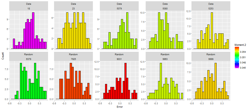
Let's see this approach in action with the values given in the question. First, let's examine a search of all denominators $n$ up to $n=10^4$.

The top row presents error histograms for the five best $n$, ordered by $n$ and colored according to their second moment: red and orange are bad; violet and blue are good. The bottom row presents error histograms for uniform random data pulled from the same range as the data and searched (independently) in the same way.
This figure is rather uninteresting: no histogram for the data looks exceptionally better than histograms for the random values.
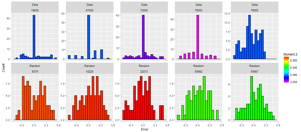
Let's extend the search. The next one goes out to $n=10^5$.

Obviously something is going on: the data histograms are remarkably better than the random ones. (The range of variances has expanded, so the colors--although comparable within this graphic--don't correspond to those in the previous graphic.) The first four have marked spikes at zero: multiplying by these denominators makes the majority of the data integral. Nothing comparable happens with the random data. And take a look at the denominators that emerge for the data: they are all multiples of $19000$. There's something special about this number!
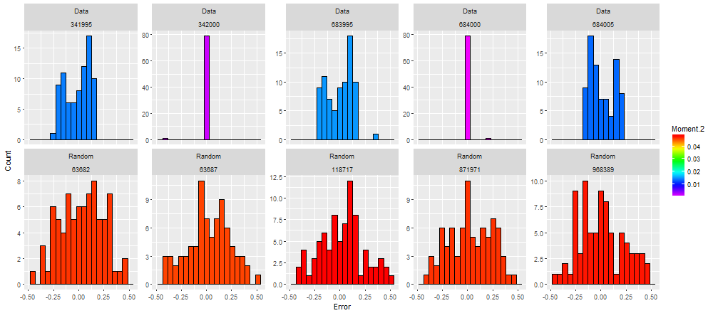
However, the spread of values even in the best data histograms shows that not all the data are whole multiples of $1/19000$. The distinct spacing exhibited in two of the histograms (for $n=57000$ and $n=76000$) suggests that a small multiple of $19000$ might do the trick. We might consider continuing our search for $n=6\times 19000, 7\times 19000, \ldots$ and see what happens. To make sure no possibility is overlooked, though, I simply prolonged the search to all $n$ up to one million ($10^6$):

The denominator $n=342000$ is the first (smallest) which makes almost all the numerators integral: only one is not. The difference between the data and the random values is striking and large.
When the original data are multiplied by this $n$, all but the first value are within $0.005$ of an integer. (The first one is $0.40$ too low.) This suggests we could retain essentially all the precision in the data by representing them as fractions with a denominator of $342000$. The numerators are
262759 263017 263286 ... 282744 282283
If this seems like too much precision, we might retreat to the smaller denominator of $n=19000$: the errors are at most $0.5/19000 \approx 3\times 10^{-5}$ and many are zero. That's $4.5$ significant digits, more than enough for most statistical calculations and visualizations.
Appendix
Here is the R code implementing the calculations and graphical displays. It begins with assigning the data to the array x (not shown, since the data already appear in the question).
library(ggplot2)
library(data.table)
analyze <- function(x, N=20, Id="", n.min=1e3, n.max=1e6) {
  error <- function(n) x*n - round(x*n)
  v <- function(n) mean(error(n)^2)
  N <- min(N, length(x))
  y <- sapply(n.min:n.max, v)
  m <- (n.min:n.max)[order(y)[1:N]]
  X <- data.table(Rank=rep(1:length(m), each=length(x)),
                  m=rep(m, each=length(x)),
                  x=rep(x, each=length(m)),
                  Moment.2=rep(y[m - n.min + 1], each=length(x)))
  X[, Error := error(m)]
  X[, m := ordered(m)]
  X[, Group := Id]
  return(X)
}
set.seed(17)
x.0 <- runif(80, min(x), max(x))
n.min <- ceiling(1/diff(range(x)))
n.min.0 <- ceiling(1/diff(range(x.0)))
for (n.max in c(1e4, 1e5, 1e6)) {
  X <- rbind(analyze(x, n.max=n.max, n.min=n.min, Id="Data"),
             analyze(x.0, n.max=n.max, n.min=n.min.0, Id="Random")
  )
  g <- ggplot(X[Rank <= 5], aes(Error, fill=Moment.2, group=Group)) +
    geom_histogram(color="Black", bins=20) +
    # facet_grid(Group ~ Rank, scales="free_x") +
    facet_wrap(~ Group + m, nrow=2, scales="free_y") +
    scale_fill_gradientn(colors=rev(rainbow(40)[1:34])) +
    ylab("Count")
  print(g)
}

