2
$\begingroup$

I trying to create a very simple forecasting routine for a time series. I am using three methods to fit and compare their accuracies. These methods are ets, auto.arima and stlf from forecast package. An example of a time series is shown below.

count <- c(231.61, 0.00, 228.70, 3197.99, 3941.62, 4400.92, 2386.03,
 311.22, 0.00, 621.96, 0.00, 414.33, 719.38, 907.70, 1005.59, 998.46,
 199.00, 298.35, 994.50, 497.01, 1013.48, 0.00, 249.86, 187.95, 1033.74,
 939.77, 382.32, 1441.69, 1284.46, 823.41, 1410.24, 2976.88, 711.86, -74.90, 
 1661.38, 1712.29, 1000.45, 769.57, 904.88, 846.33, 846.33, 1501.34, 
 1696.61, 1615.40, 630.88, 1090.95, 1256.66, 1043.50, 1838.87, 1838.85, 
 212.39, 0.00, 171.31)

d.ts <- ts(count, start = c(2015, 5), freq = 12)

And, here are how I am doing every fitting.

library(forecast)

fit.ets <- ets(d.ts)
fit.stl <- stlf(d.ts, robust = T, s.window = "periodic")
fit.arima <- auto.arima(d.ts, stepwise = F, approximation = F)

When I try to plot the fitted values and original values, I get the following plot. Plotting fitted vs. original values

plot(fit.ets$x, col = "red")
lines(fitted(fit.ets), col = "blue")

produces the following plot. ETS Original vs. Fitted

It looks like as if there is a 1-lag between the original and fitted values. Plotting auto.arima fit

plot(fit.arima$x, col = "red")
lines(fitted(fit.arima), col = "blue")

produces similar results. AUTO.ARIMA Fitted vs. Original Is this a normal behaviour? If it is, what is the cause?

$\endgroup$

2 Answers 2

2
$\begingroup$

Yes, this is normal. Look at your fitted models:

> fit.ets
ETS(A,N,N) 

Call:
 ets(y = d.ts) 

  Smoothing parameters:
    alpha = 0.9999 

  Initial states:
    l = 229.4376

ets() fits a model with additive error, no trend and no seasonality. This is (the state space form of) Single Exponential Smoothing,

$$ \hat{y}_t = \alpha y_{t-1}+(1-\alpha)\hat{y}_{t-1}.$$

Note also that $\alpha=0.999$, so ets() thinks that your series is almost a random walk. (A random walk, $y_t=y_{t-1}+\epsilon_t$, would correspond to $\alpha=1$, but ets() won't fit this, because it is nonstationary.) Thus, it essentially believes that the best forecast is the last observation. The in-sample fit therefore is almost just the previous observation.

Similarly,

> fit.arima
Series: d.ts 
ARIMA(2,0,0) with non-zero mean 

Coefficients:
         ar1      ar2       mean
      0.7457  -0.3483  1027.7672
s.e.  0.1275   0.1289   168.2384

auto.arima() fits an AR(2) process with a mean,

$$ \hat{y}_t = \phi_1y_{t-1}+\phi_2y_{t-2} + c, $$

again with pretty large coefficients of $\phi_1=0.75$ and $\phi_2=-0.35$. Very roughly speaking, next month's forecast is 75% determined by this month's observation.

Both ets() and auto.arima() believe that there is no trend or seasonality to your data, and based on the plot, I would agree. Either model may produce good forecasts. In particular, the random walk is not a completely unrealistic benchmark. You may also want to look at other simple methods like the overall mean or median. If you have any external drivers, you could include these in a causal forecasting model. Best to use a holdout sample and see how the models compare on that.

$\endgroup$
0
$\begingroup$

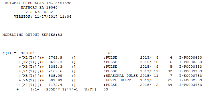
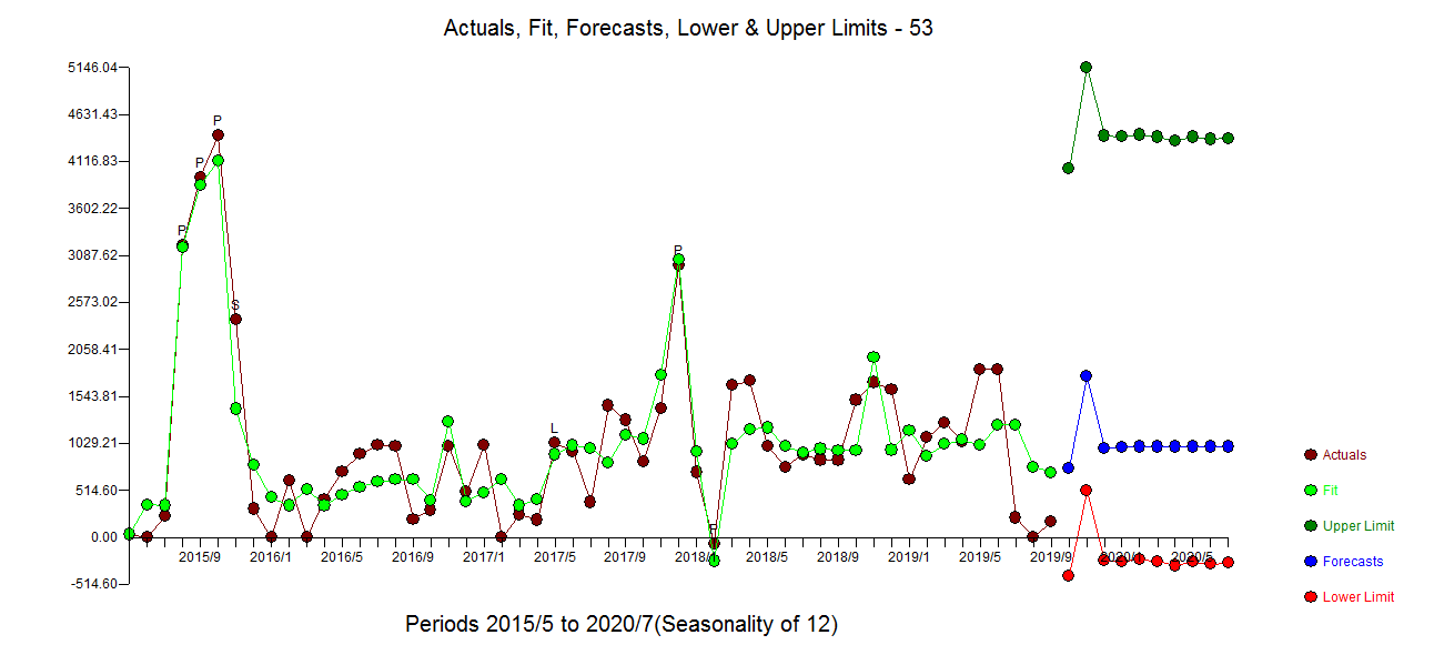
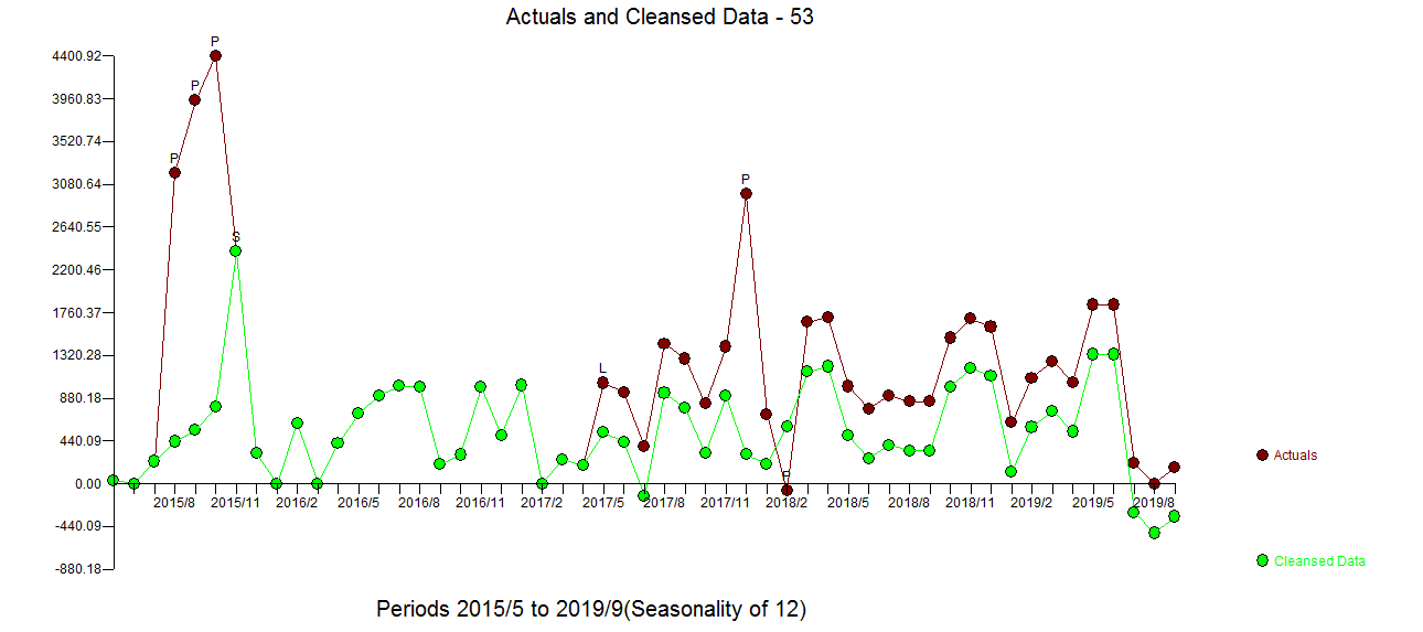
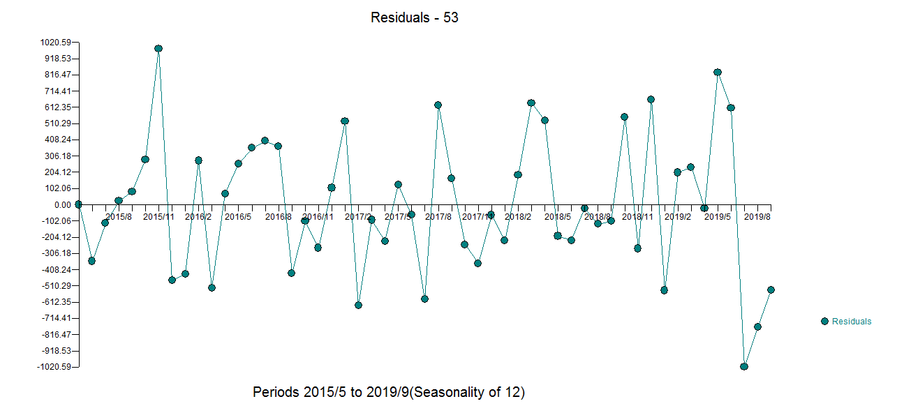
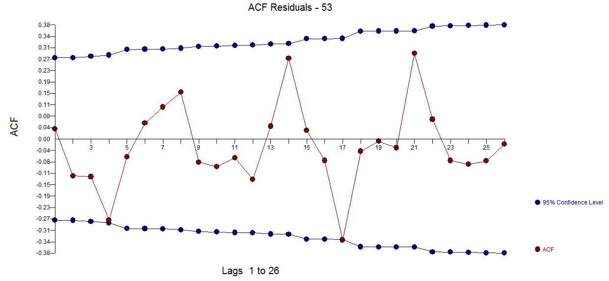
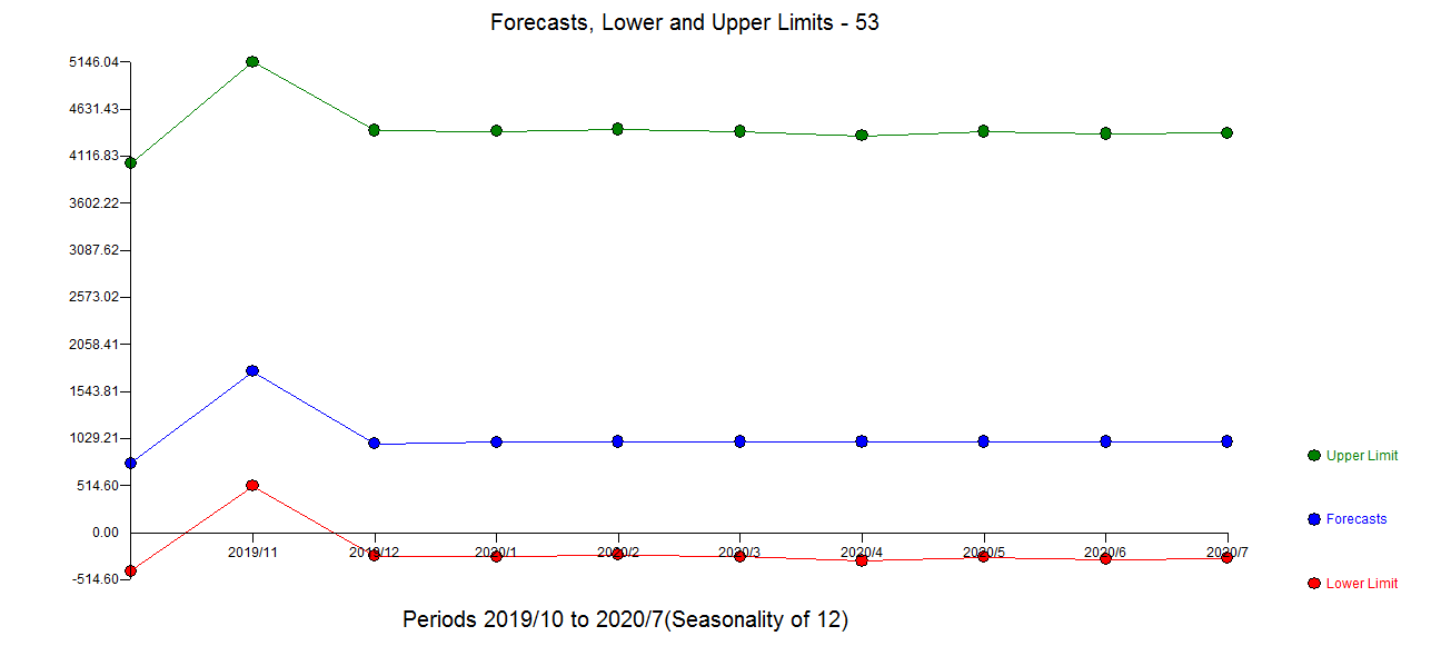
When you have data that has been effected by external factors creating model identification ambiguity a nuanced approach is important/critical to identify those effects and isolate them in order to form a more useful model. The eye (like statistical tools) works better when it is not occluded. With your data a few one time anomalies and a level shift one gets enter image description here a similar model form is the same as @STEPHAN and different forecasts coming off the recent level shift. enter image description here . The plot of the cleansed and actual is here enter image description here . The plot of the residuals enter image description hereand the acf of these residuals description here enter image description hereis a mandatory exercise to test the assumptions underlying the proposed model . The forecast plot is here enter image description herewith confidence limits reflecting possible future anomalies.

$\endgroup$

Your Answer

By clicking “Post Your Answer”, you agree to our terms of service and acknowledge you have read our privacy policy.

Not the answer you're looking for? Browse other questions tagged or ask your own question.