Draw from random distributions so that sum of values is fixed

Question

I want to draw tuples of $N$ random numbers $v_{ij}$ with $i=1,..,N$ the tuple index and $j$ the repetition of the experiment.

The sum of all random numbers in a tuple should be constant $\forall j \sum_i v_{ij}=S$.

The expectation and variance of each $i$-th index in the tuples should be known $\mathrm{E}_j(v_{ij})=e_i>0, \sum_i e_i=S$ and $\mathrm{Var}_j(v_{ij})=v_i$.

The values should be non-negative $0\le v_{ij}\le S$.

The distribution of $v_{ij}$ for each $i$ should look as normal-distributed like as possible.

I'm aware that the condition that the sum is fixed will make them not independent. If possible I would like to distribute the correlations between different indices $i$ as equally as possible.

My idea:

I draw $N-1$ binomially distributed random numbers, scale them to match $e_i$ and $v_i$, then set the last value in the tuple to $S$ minus the sum of these distributed numbers.

However, the variance of the last index value in the tuples is usually much larger than desired and difficult to set independently and I cannot guarantee that the values in the last index stay within the bounds $[0,S]$.

Example: $N=4,e_1=10,e_2=20,e_3=40,S=100$.

The answers of Simulation involving conditioning on sum of random variables didn't help me because they seem to be special to the problem presented there and not applicable to my conditions.

How can I achieve what I want?

Answer 1

You can get close to what you want by using a singular normal distribution - and if you use equal variances you will get equal negative pairwise correlations.

Using the transformation method (see guy's solution here r - pick 10 random numbers from standard normal distribution whose sum equals 5 for an example), we can find the covariace matrix (I've chosen 3 as the variance) $$ \Sigma = \pmatrix{\ \ 3 & -1 & -1 & -1 \\ -1 & \ \ 3 & -1 & -1 \\ -1 & -1 & \ \ 3 & -1 \\ -1 & -1 & -1 & \ \ 3}.$$

Now we can use singular value decomposition (SVD) to generate the variates (see whuber's code here - Generating samples from singular Gaussian distribution)

Modifying whuber's code to suit your problem, we have:

library(MASS)

# Specify the mean vector for the multinormal distribution
mu <- c(10,20,30,40)

# Use equal variances, which leads to equal correlations
# of -1/3 among all pairwise combinations
sigma <- matrix(c(3.0,-1,-1,-1,-1,3.0,-1,-1,-1,-1,3.0,-1,-1,-1,-1,3.0),4,4)    # Covariance matrix is singular

n <- dim(sigma)[1]
s <- svd((sigma + t(sigma))/2) # Guarantees symmetry
s$d <- abs(zapsmall(s$d))
m <- sum(s$d > 0)

# Generate normals in the lower dimension
n.sample <- 100000   # Number of realizations
x <- matrix(rnorm(m*n.sample),nrow=m)

# Embed in the higher dimension and apply square root
# of sigma obtained from its SVD
x <- rbind(x, matrix(0, nrow=n-m, ncol=n.sample))
y <- s$u %*% diag(sqrt(s$d)) %*% x + mu

# Prepare data for plotting
library(data.table)
x1 <- data.table(y[1,])
x2 <- data.table(y[2,])
x3 <- data.table(y[3,])
x4 <- data.table(y[4,])

# Add in label
x1$var <- 'x1'
x2$var <- 'x2'
x3$var <- 'x3'
x4$var <- 'x4' 

all <- rbind(x1,x2,x3,x4)

# Plot histograms of the four components
ggplot(all, aes(V1, fill = var)) + geom_density(alpha = 0.9)

# Check a few totals 
sum(y[1:4,1])
sum(y[1:4,2])
sum(y[1:4,10])
sum(y[1:4,n.sample])
sum(y)

# Check to see how close the empirical correlations are 
# to negative 1/3
cor(y[1,],y[2,])
cor(y[1,],y[3,])
cor(y[2,],y[3,])

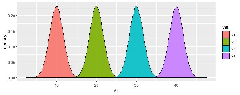
Here is the chart:

Here is output verifying the sum requirement for a few realizations and some of the empirical correlations:

> sum(y[1:4,1])
[1] 100
> sum(y[1:4,2])
[1] 100
> sum(y[1:4,10])
[1] 100
> sum(y[1:4,n.sample])
[1] 100
> sum(y)
[1] 1e+07
> 
> # Check to see how close the empirical correlations are 
> # to negative 1/3
> cor(y[1,],y[2,])
[1] -0.3294876
> cor(y[1,],y[3,])
[1] -0.331753
> cor(y[2,],y[3,])
[1] -0.336657

If you want to specify non-equal variances among your components, you will have a different covariance matrix. You will also not have equal pairwise correlations.

Part 2 - Unequal Variances

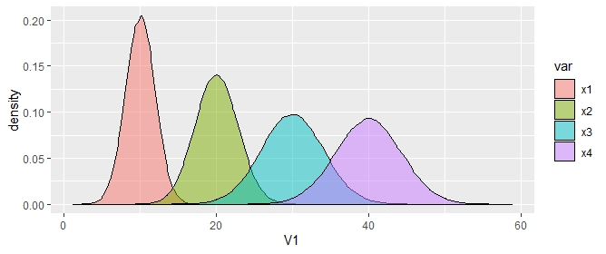
Suppose we want variances of 2, 3, 5, and 6.

If you use the following covariance matrix,

sigma <- matrix(c(3.7838,-0.4865,-1.3514,-1.9459,-0.4865,7.9054,-3.0405,-4.3784,-1.3514,-3.0405,16.5541,-12.1622,-1.9459,-4.3784,-12.1622,18.4865),4,4)    # Covariance matrix is singular

You will get the following chart:

If this is of interest, I will post more on how to find the covariance matrix.