Distribution of the $90$th percentile of a geometric brownian motion simulation

Question

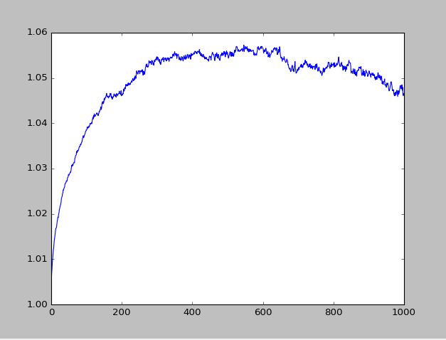
I have run a simulation of a geometric brownian motion. The simulation runs from $t=0$ to $T=1000$. I generate $10000$ paths. For every moment for $t=1,2,3,\ldots, 100$ I calculate the $90$th percentile of the simulated paths. When I plot these points, depending on the used parameters, the curve that is produced is concave or convex. Please check the figure for an example.

When $\sigma$ is large relative to $\mu$, the curve of the $90$th percentile is concave (as above), and when $\sigma$ is small relative to $\mu$ the curve is convex. Is there any analytic formula for the distribution of percentiles of the GBM between two time instances? Also, is there an analytic or heuristic way to predict the shape of the 90th percentile (or any other percentile)? Thanks for the help.

Answer 1

The GBM's distribution at any given point is $$\ln x_t= \mathcal N(\mu t,t\sigma^2)$$ Hence the 90th percentile would be $$g(t)=\exp\left(\Phi^{-1}(\mu t,t\sigma^2,0.9)\right)=\exp\left(\mu t +\sqrt t \sigma \Phi^{-1}(0.9)\right)$$ where $\Phi^{-1}()$ is the normal or standard normal inverse CDF. This curve is certainly concave and smooth for any $\mu$ and $\sigma^2$.

Consider the second derivative: $$g''(t)=\left(\left(\mu+\frac 1 2 \sigma \Phi^{-1}(0.9)t^{-1/2}\right)g(t)\right)'=\\ \left(-\frac 1 4 \sigma\Phi^{-1}(0.9) t^{-3/2}+\mu+\frac 1 2 \sigma \Phi^{-1}(0.9)t^{-1/2}\right)g(t)=\\ \left(\frac 1 4\sigma \Phi^{-1}(0.9)(2- 1/t)t^{-1/2}+\mu\right)g(t) $$ Since $g(t)>0$, the $g''(t)>0$ only when the following holds: $$\frac 1 4\sigma \Phi^{-1}(0.9)(2- 1/t)t^{-1/2}+\mu>0$$ In other words this is the condition of convexity. It can be shown that it holds at sufficiently large $t$. So, the true percentile is concave at small $t$, and convex at large $t$.

You can see why this happens intuitively. At small $t$ the exponent is close to linear $e^x\sim 1+x$. Hence the only source of nonlinearity comes from the square root of time term in $g(t)$, which is concave. When $t$ is sufficiently large, the exponent, which is convex, starts to dominate and the percentile curve becomes convex.

The reason why you think that the entire curve switches convexity is due to imprecision of your Monte Carlo simulation. For instance, what appears to you as switching between convexity and concavity could be that you are in a sense looking at different parts of the curve. When you're playing with $\mu$ and $\sigma$ you're effectively changing the scale of your plot on $t$ axis. So, sometimes that inflection point can be to the right and sometimes to the left of you plot.

Now, your curve is an empirical 90th percentile, and it's a random curve as such. It will not have a derivative at any point in an ordinary sense, like @whuber mentioned. Hence, in an ordinary sense, i.e. second derivative's sign, it cannot be concave or convex. You'd have to define some measure of convexity for a random curve that doesn't have derivatives in order to judge whether your curve is concave or convex. Obviously, your measure should reconcile with the result I gave you based on theoretical properties of the percentile of GBM. Otherwise, it will not be a sensible measure, if it's not working even in a tractable case where the analytical solution is known.

Answer 2

I am a little unclear on what the graph is. You mention calculating 100 moments, but I presume this is the 90th percentile boundary for the value of the path. ALso, i presume this is the upper 90th percentile boundary; assumedly there is a lower 90th to go with it?

If I understand what you are doing right, the shape just shows which term is dominating. If $\mu$ (the drift) is large and the volatility is really close to zero, it should look like $e^{rt}$ since there is exponential growth. But, if $\mu$ is zero,and $\sigma$ is a realistic number, what you mwould see is the bounds growing as $\sqrt t$.