How to calculate the standard deviation for a Gaussian Process?

Question

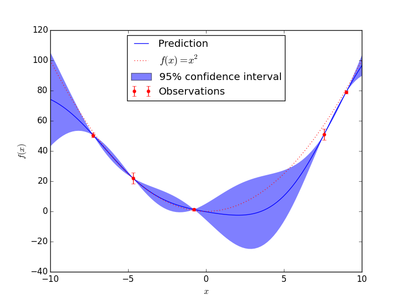
I am quite new to Gaussian processes. A Gaussian Process looks like the following:

Where the dark blue line denotes the mean, and the filled-area denotes the mean+std and mean-std respectively.

From what I know, we can calculate the predicted mean function as follows

• $K$ denotes the kernel used
• $x_*$ denotes the x-coordinate to be predicted
• $x_d$ denotes all the 'training data'/previously sampled data):

$$ m( y_* | y_d) = \mu(x_*) + K(x_*, x_d) K(x_d, x_d)^{-1} (y_d - \mu (x_d)) $$

and the covariance function as follows:

$$ C(y_* | y_d) = K(x_*, x_*) - K(x_*, x_d) K(x_d, x_d)^{-1} K(x_d, x_*) $$

As I am currently new to Gaussian processes and try to understand the process before going into implementations, I started working through this blog-post. Here, the author calculates the following to end up with the standard-deviation:

K_ss = kernel(Xtest, Xtest)
K_s = kernel(Xtrain, Xtest, param)
K = kernel(Xtrain, Xtrain, param)

L = np.linalg.cholesky(K + 0.00005*np.eye(len(Xtrain)))
Lk = np.linalg.solve(L, K_s)

s2 = np.diag(K_ss) - np.sum(Lk**2, axis=0)
stdv = np.sqrt(s2)

My initial thought was that the covariance-function $C(y_* | y_d)$ can be used to calculate the standard deviation for each sampled data point in the above graph. However, looking at the code, I don't quite understand how this is done.

So my question is: How is the standard deviation calculated? And how can I then arrive at a graph like the above one?

Answer 1

The closed form equation for the predicted covariance inverts $K(x_d, x_d)$. However, using the Cholesky decomposition is faster and more numerically stable than directly taking the inverse. You can see the procedure laid out in Algorithm 2.1 of Gaussian Processes for Machine Learning. However, they don't show why they're equivalent, so I'll sketch it out here.

First

The closed-form equation gives a $n$ x $n$ covariance matrix for $d$ test points. The code only cares about it's diagonal. $K(x_*, x_*)$ is the $n$ a $n$ prior covariance between the test points, but the code extracts

np.diag(K_ss)

Note that

np.sum(Lk**2, axis=0)

is equivalent to:

np.diag(Lk.T @ Lk)

In other words,

Lk.T @ Lk 

is somehow equivalent to

$$ K(x_*, x_d) K(x_d, x_d)^{-1} K(x_d, x_*) $$

The Cholesky decomposition of $K$ produces a lower triangular matrix $L$ with real positive diagonal entries such that

$$K = LL^T$$

Let $k_s = K(x_d, x_*)$ so that the least squares (np.linalg.solve) step outputs: $$L_k = (L^TL)^{-1}L^Tk_s$$

$(AB)^T = B^TA^T$, $(AB)^{-1} = B^{-1}A^{-1}$, and $(A^{-1})^T = (A^T)^{-1} = A^{-T}$ , so

\begin{align} L_k^TL_k &= k_s^T L [(L^TL)^{-1})]^T(L^TL)^{-1}L^Tk_s\\ L_k^TL_k &= k_s^T L (L^{-1}L^{-T})^TL^{-1}L^{-T}L^Tk_s\\ L_k^TL_k &= k_s^T L L^{-1}L^{-T}L^{-1}L^{-T}L^Tk_s\\ L_k^TL_k &= k_s^T L^{-T}L^{-1}k_s \end{align}

From the definition of the Cholesky decomposition: $$ K^{-1} = (LL^T)^{-1} = L^{-T}L^{-1}$$

Therefore:

$$ L_k^TL_k = k_s^T K^{-1} k_s $$

Finally, note that in the code, they add a small diagonal element to the training covariance so that: $$K = K(x_d, x_d) + \sigma_n^2I$$.

The small diagonal element represents an estimate of the observation noise. That is, we assume that the observations $y$ are normally distributed with mean $f(x)$ and variance $\sigma_n^2$. Numerically, this helps to guarantee that the training covariance is positive definite.