How do I interpret this residual diagnostics plot?

Question

I am just learning to understand how to utilize residual plots to improve regression models. It seems like the following residual vs. fitted plot is hugely problematic as it has a pattern. But how do I go about identifying the most likely causes for such an issue?

The following is a residual vs fitted plot when the dependent variable is log-transformed. I guess the same issue of pattern persists:

Answer 1

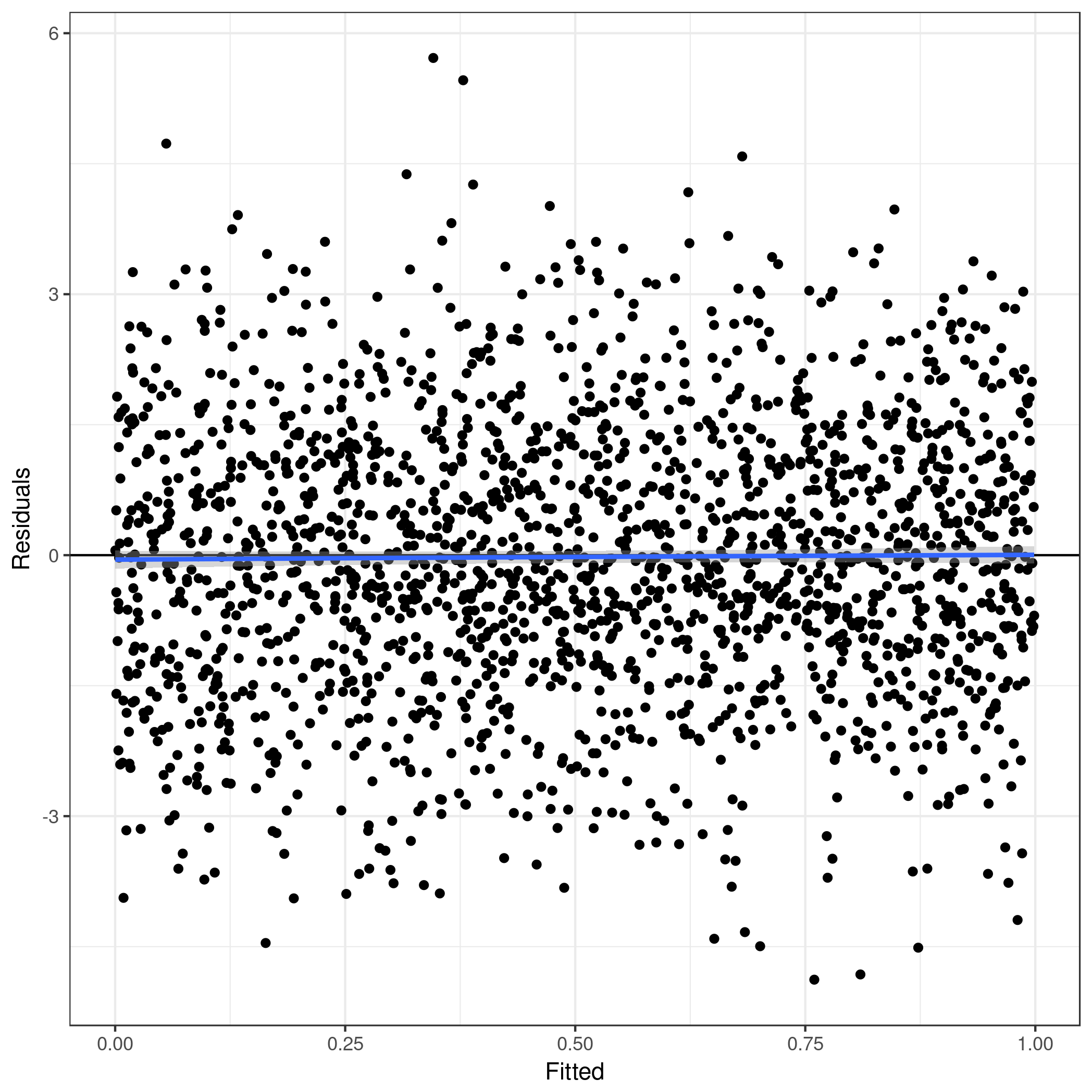
A "good" residuals vs fitted plot for a linear model might look something like this

library("ggplot2")
theme_set(theme_bw())
set.seed(1)
df <- data.frame(e = rnorm(2000, 0, sd = 1.5),
                 yhat = runif(2000))
ggplot(df, aes(x = yhat, y = e)) +
  geom_abline(intercept =  0, slope = 0) +
  geom_point() +
  geom_smooth() +
  labs(y = "Residuals", x = "Fitted")

Notice

• how the residuals are spread evenly around 0 throughout the range of the fitted value,
• the residuals have the same variance --- they are evenly spread the ~ the same distance either side of zero throughout the range of the fitted values (i.e. there's about the same number of residuals $>|3|$ for example at each location on the x-axis.)
• there is no strong systematic pattern in the residuals; the blue line is similar to the red one in your plot and is a scatterplot smoother showing pattern in the mean of residuals.

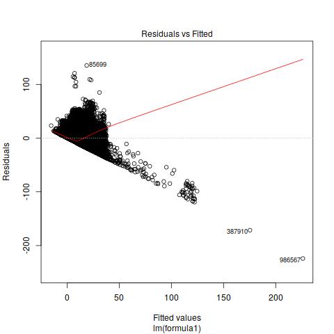
In your plot we notice two signifant problems:

1. There is clear non-constant variance. The spread of the residuals towards the left of the plot is much less than the spread towards the right of the plot.
2. There is substantial bias in the estimated values; all the residuals are negative above a fitted value of ~40. Similarly, all the residuals at small fitted values (towards the left of the plot) are positive.

These suggest that

1. the conditional distribution of the response is not Gaussian. In other words, once you account for the effects on the response of your predictor variables (covariates), the response is not normally distributed.

From your reply to @Isabella, an immediate problem is that the response variable is number of days to get a loan. This is unlikely to be conditionally distributed Gaussian because you can't have a negative number of days; the distribution of the response is bounded at 0. Typically, such count data have a non-constant mean-variance relationship; the variance (spread of data about the mean) increase as the mean value increases.

Counts like this are typically modelled as being conditionally distributed Poisson, using a Generalised Linear Model (GLM) with a Poisson family and log link. This is often a useful starting point but other distributions are also used for integer counts that can account for more complexity in the observed counts than can be accounted for in the Poisson.

If your response is not an integer number of days (2.4 days is an allowed value) then you would need a distribution that has support on the positive real values (any value > 0). Such distributions include the Gamma distribution, which also can be fitted as a GLM.

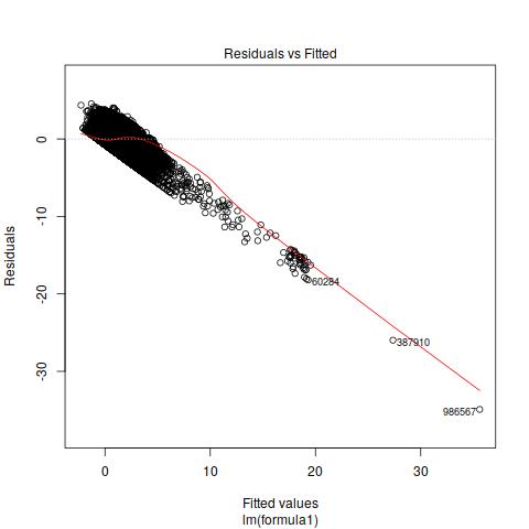
If you do not have an 0 day values in the data set, then you could quickly try to fix the problem of the wrongly assumed mean-variance relationship by applying a log-transformation to the response variable (lm(log(y) ~ x1 + x2) in pseudo code) and see if that improves things. But typically one would prefer a GLM-like model so that one can estimate the mean of the response directly rather than the mean of the log of the response.

From the limited amount of information you have provided, there is little more than I can say beyond the above.