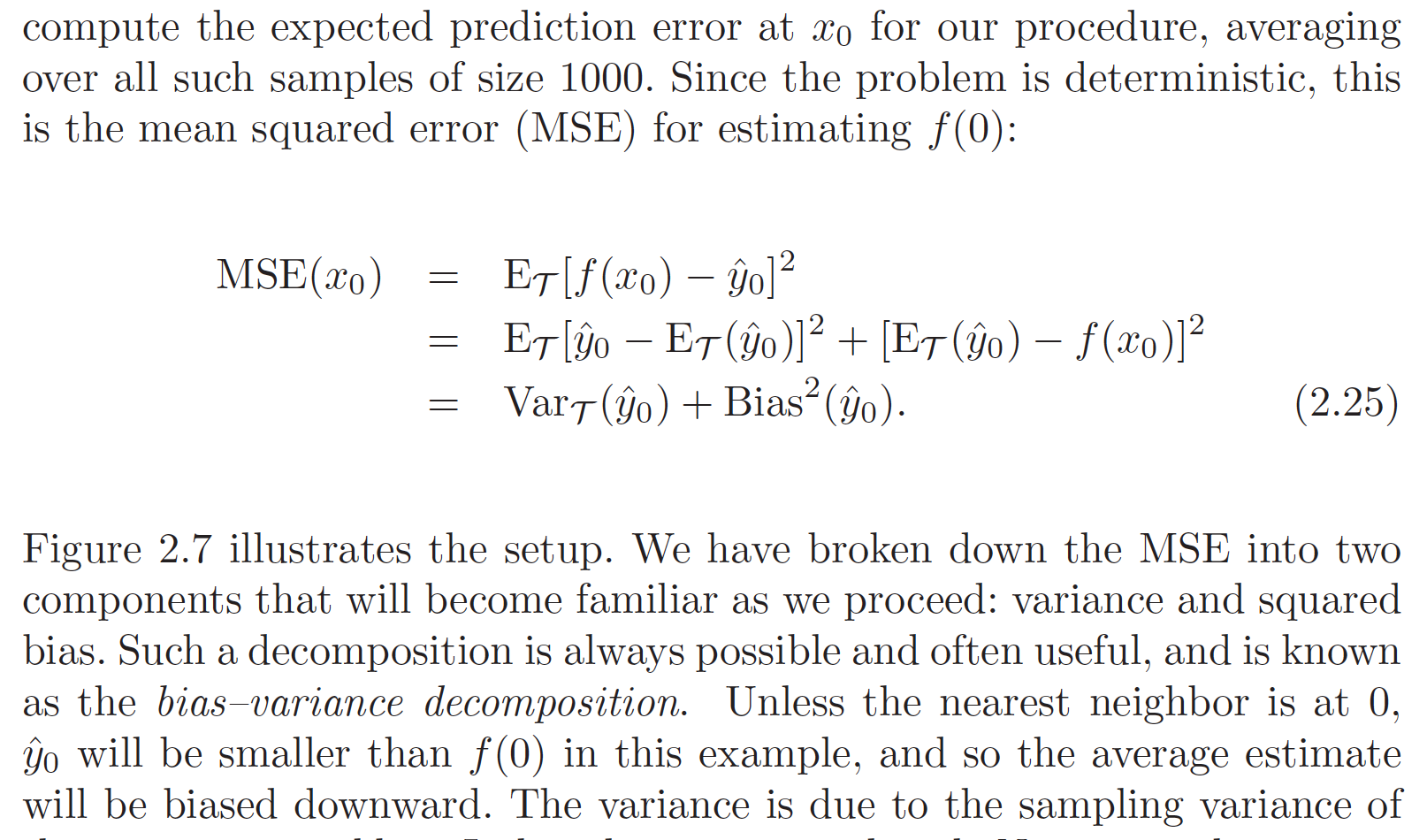
I understand how the bias-variance decomposition was done, but I'm not sure what the author means when he says "Unless the nearest neighbor is at 0, $\hat{y}_{o}$ will be smaller than f(0) in this example, and so the average estimate will be biased downward." I understand that since any other x point will return a $\hat{y}_{o}$ value lower than f(0) that the average estimate will always be less, but how was that conclusion come about from the bias-variance decomposition?
1 Answer
I think the reason the authors introduced the bias-variance decomposition is that for this specific example, the impact of the curse of dimensionality is more significant on bias than it is on variance.
Here is the authors' example, $Y=e^{-8\left\|X\right\|^{2}}$ whose maximum is always 1 at $X=0$. They are trying to estimate $y_{0}$ at the test-point $x_{0}=0$ by using 1-nearest-neighbor. Below is the decomposition.
$$MSE(x_{0}) = E_{\tau}[\hat{y}_{0} - E_{\tau}(\hat{y}_{0})]^{2} + [E_{\tau}(\hat{y}_{0})-f(x_{0})]^{2}$$ $$=Var_{\tau}(\hat{y}_{0}) + Bias^{2}(\hat{y}_{0})$$
Suppose they have a data and the data includes observation $y_{0}$ and $x_{0}$, then their estimate for $y_{0}$ is unbiased because the known nearest neighbor to $x_{0}$ is the goal itself, so $\hat{y}_{0} = y_{0}$. But this phenomenon rarely happens, or this probability is really low.
Most of the time they didn't have $y_{0}$ and $x_{0}$. For the estimate of $y_{0}$, they have to dig into the training data, find the closest $X$ to $x_{0}$, which can be denoted by $X^{*}$, and use observed $e^{-8\left\|X^{*}\right\|^{2}}$ (authors mentioned there were no measurement error) to estimate $y_{0}$. All these estimates are smaller than the maximum, the true $y_{0}$. Moreover, as the X's dimension $p$ increases, the chance for all data points to scatter further away from the origin and closer to the boundary also increases. This trend has been discussed by the authors in page 23. Therefore we expect to see smaller estimate (smaller $E_{\tau}(\hat{y}_{0})$) as $p$ goes up, the bias is downward. This is the connection between bias and the dimension $p$. In their Figure 2.7 page 25, you can see the bottom-right plot shows an increasing squared bias trend. Since as $p$ increases bias is a smaller negative value, its square is a larger positive value.
They also mentioned the trend of variance as $p$ increases. They said this was a 'highly contrived' example. So I think for this specific example, the downward trend of bias due to the curse of dimensionality, or the upward trend of squared bias, is more obvious. According to that plot, the trend of variance is not as obvious as the squared bias.
Later the authors mentioned another example of the situation that variance 'dominates' over bias. You can see in the right plot of Figure 2.8 the trend of increasing variance is way more obvious than the trend of squared bias as $p$ increases.


