decompose will decompose any time series, whether there is a seasonal signal or not. It does not do, e.g., a significance test, and quit if there is no discernible seasonal signal. It is kind of dumb that way.
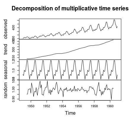
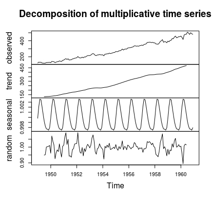
Note the $y$ axes of your two decomposition plots. In the decomposition of the original data, the seasonal component goes from 0.80 to 1.20, so we have roughly a 20% seasonal signal. When you decompose the already-decomposed data, the seasonal component goes from 0.998 to 1.002, so we have a roughly 0.2% seasonal "signal". I'd say this is consistent with no remaining seasonality in the decomposed series. A number of standard seasonality tests are of the same opinion:
library(forecast)
nsdiffs(deSeas,test="seas")
# [1] 0
nsdiffs(deSeas,test="ch")
# [1] 0
nsdiffs(deSeas,test="hegy")
# [1] 0
nsdiffs(deSeas,test="ocsb")
# [1] 0
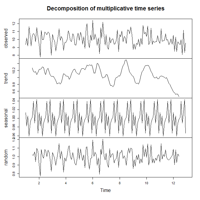
When you are faced with some hard-to-understand statistical behavior, it is often instructive to check how your method performs on completely random data. In the present case, you can see that decompose() will happily decompose completely unseasonal random noise. However, note again the $y$ axis on the seasonal component in the plot:

set.seed(1)
foo <- ts(rnorm(144),frequency=12)+10
plot(decompose(foo,"multiplicative"))
One difference between plot(decompose(deSeas,"multiplicative")) and plot(decompose(foo,"multiplicative")) is visible: deSeas gives a far more regular seasonal component. As such, there may be some tiny remaining seasonality. I would assume that the true AirPassengers data generating process is not completely multiplicative, so even after multiplicative deseasonalization, some very little signal remains.
One could investigate this by generating some data with a true multiplicative DGP, then check whether decompose() correctly removes the seasonality, leaving something that, when decomposed again like the foo series, shows a seasonal component that is periodic but noisy.
