The Cliff's delta statistic (or Success Rate difference):
$\delta = Pr(y_{i} >x_{j}) - Pr(y_{i}<x_{j})$
is the difference between the probability of $y_i$ greater than $x_j$ - with $y_i$ and $x_j$ randomly chosen in their respective groups - and the probability of the inverse.
It is in all respects a population parameter, but it is not a location measure such as a mean, a median, or an M-estimator. It is a stochastic dominance parameter. So the meaning of its scores is to be referred to a difference between probabilities and not between means.
The interest in delta arises by realizing that the distributions' identity assumption is often impractical, and by observing that the Wilcoxon-Mann-Whitney test - the best-known approach to comparing two independent groups - can give a p-value of 0.05 even when the population means are identical, if variances differ (Behrens-Fisher problem). As a matter of fact, according to Wilcox (2005) it should not at all be applied to test unequal variances because it uses a standard error derived under the assumption that the two groups have identical distributions.
For better understanding the relationship between a difference in probabilities and a difference in means as an effect-size measure, Neuhäuser, M., Lösch, C., & Jöckel, K.-H. (2007) suggest a comparison with the special case of normal distributed data with means $\mu_1$ and $\mu_2$ and SDs $\sigma_1$ and $\sigma_2$. Let be:
$ P=\Phi$ $\Bigl(\frac{\mu_1 - \mu_2}{\sqrt (\sigma_1^2 + \sigma_2^2)}\Bigr)$
"where $\Phi$ is the cumulative distribution function of the standard normal distribution (Reiser and Guttman (1986)). Since $\Phi(t) = \frac12$ if and only if
$t = 0$, $\mu_1$ = $\mu_2$ is equivalent to $P = \frac12$, but standard deviations $\sigma_1$ and $\sigma_2$ can differ. Furthermore, $P$ is smaller than $\frac12$ if $\mu_1 > \mu_2$ and larger if $\mu_1 < \mu_2$. In general, the observations in group 1 tend to be larger in comparison to those of group 2 if $p < \frac12$. In the case of $P > \frac12$ the observations in group 1 tend to be smaller than those of group 2. If $P = \frac12$, neither group generally has larger values than the other and $Pr(X >Y ) = Pr(X <Y )$ holds (Delaney and Vargha, 2002)".
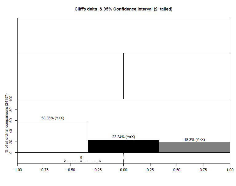
Would the 58.93% (Y < X) indicate that the Y group "scored" 58% less than that X group?
In your case, the d value should be determined as follows: 18.3 - 58.36 = -40.06.
The stochastic dominance is measured by matching each observation in the first group with each other in the second one and assigning a value of $1$ if it is greater, a value of $0$ if it is equal and a value of $-1$ if it is smaller.
The resulting matrix, of $n_1n_2$ values, is called dominance matrix. The function orddom::dm() prints it. The average value of all the dominance matrix entries is $d$, the sample value of Cliff's delta.
And what would a negative Cliff's D indicate?
As for its sign, being a difference, it simply depends on the order in which the groups are entered in the function's call. If you switch $X$ and $Y$, the delta value will become positive, 40.06. The sign only says which group dominates the other (whether Disagree is prevailing on Agree or viceversa). However, the p value goes with the absolute value.
The R's orddom::delta_gr() function
Maybe due to a bug, sometimes not every part of the output is correctly printed by the delta_gr() function (orddom package in R). Your graph shows these symptoms. This can make harder the groups' identification and so the result's interpretation.
To circumvent it, in calling the function, try inverting the position of variables $X$ and $Y$. You should get the complete output. Moreover, I suggest to pass the x.name="XNAME" and y.name="YNAME" parameters to the delta_gr() function, to clarify the output.
You should get something like:
"There is a 18.3% chance that a case randomly chosen from group Y (YNAME) has a higher score than a randomly chosen subject from group X (XNAME), as compared to a 58.36% probability for the reverse, resulting in a success rate difference (i.e. an estimated delta value of) -0.4006.
There is a 95% probability that the 'true' delta value can be found between CI (lower) = ........ and CI (higher)= ............" in the top area.
In the second row, you'd get some other information, such as the groups' size, delta, s (delta's standard dev), z score of delta, the p-value for statistical significance of delta (if the probability difference between Strongly Disagree and Strongly Agree is statistically significant), Cohen's d, plus two histograms with density curves overimposed.
On the bottom, a 95% CI of delta is graphed. The group entered as Y should be the experimental group (bugs aside) and as delta=Y−X, a positive delta means that Y is the dominant group, with the CI bar lying on the right side. If the interval does not span the zero, the difference is significant at alfa=0.05.
Above the bar, the histogram resembles a scales: the bar works as a needle which goes toward the heavier group.
To summarize, the Cliff's delta and the Brunner-Munzel test are sometimes preferred to the Wilcoxon Mann Whitney, since they don't rely on the distribution's identity assumption. Both of them can handle ties.
On the other hand, whenever the distribution's identity assumption is met, the WMW can be used as a distribution-free test of difference between means or medians.
Results of a comparison between WMW, Brunner-Munzel and Cliff's tests by mean of simulations can be found in Neuhäuser, M., Lösch, C., & Jöckel, K.-H. (2007). The Chen–Luo test in case of heteroscedasticity.
References:
J. Romano, J. D. Kromrey, J. Coraggio, J. Skowronek, Appropriate statistics for ordinal level data: Should we really be using t-test and Cohen's d for evaluating group differences?
Cliff, N. (1993). Dominance statistics: Ordinal analyses to answer ordinal questions. Psychological Bulletin, 114, 494-509.
Wilcox, R.R., 2005. Introduction to Robust Estimation and Hypothesis Testing. Third ed. Elsevier, San Diego, CA.

