Non-parametric alternative to simple t-test

Question

I have five numeric variables of two populations (each of them with 60 individuals) and for each of those five variables I want to know if there is difference in the means.

I was trying to use a simple t-test for this (the t.test R function), but let me explain my concerns to see if it's possible.

One variable of one population do not pass the Shapiro normality test.

Any of the five variables passed Levene's test for 0.05, only one for 0.01 (but is the one containing the not normal distribution in one variable).

Even with all that, would it be a good choice to use the t-test to evaluate the means? What could be a non-parametric alternative that suits my problem?.

Answer 1

Let's look at one variable at a time. As I understand it you have $n_1 =60$ observations from Population 1 which is distributed $\mathsf{Norm}(\mu_1, \sigma_1)$ and $n_2 =60$ observations from Population 2 which is distributed $\mathsf{Norm}(\mu_2, \sigma_2).$

You want to test $H_0: \mu_1 = \mu_2$ against $H_a: \mu_1 \ne \mu_2.$ You could use a 2-sample t test. Unless you have prior experience with such data indicating that $\sigma_1 = \sigma_2,$ it is considered good practice to use the Welch (separate-variances) t test, which does not require $\sigma_1 = \sigma_2.$

Specifically, suppose you have the following data:

sort(x1); summary(x1); sd(x1)
 [1]  78.0  78.5  80.1  80.9  87.2  88.8  89.0  90.1  90.7  92.6  92.9  93.7  94.5  97.3  98.3
[16]  98.3  98.6 100.5 100.9 101.1 101.8 101.9 103.2 103.4 104.0 104.1 104.6 104.9 105.1 105.4
[31] 105.8 107.2 107.6 108.1 108.1 108.2 108.7 109.6 109.6 112.0 112.2 112.7 114.0 114.1 114.7
[46] 114.8 116.6 117.0 118.0 118.4 118.6 119.2 123.1 124.1 124.7 125.5 127.4 127.7 136.4 138.2

   Min. 1st Qu.  Median    Mean 3rd Qu.    Max. 
   78.0    98.3   105.6   106.2   114.7   138.2 
[1] 13.55809

.

sort(x2);  summary(x2);  sd(x2)
  [1]  65.3  70.1  76.1  76.8  80.9  81.3  82.4  82.5  84.9  85.0  85.6  86.6  87.7  88.6  89.4
 [16]  89.7  90.3  91.9  92.2  92.5  93.0  93.0  93.5  94.0  94.4  96.1  96.4  96.9  97.3  97.6
 [31]  98.5  98.9  99.7  99.9 100.2 101.3 101.5 101.7 103.3 103.4 103.5 103.6 104.5 104.7 106.0
 [46] 106.2 107.2 107.7 109.2 109.3 110.5 110.7 110.9 111.1 111.3 113.8 114.9 115.2 118.1 118.9

   Min. 1st Qu.  Median    Mean 3rd Qu.    Max. 
  65.30   89.62   98.05   97.30  106.05  118.90 
[1] 11.89914

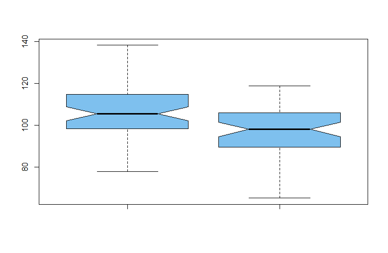
boxplot(x1, x2, notch=T, col="skyblue2", pch=19)

There are no outliers in either sample and samples seem roughly symmetrical. The notches in the sides of the boxplots are approximate nonparametric confidence intervals, here indicating that the population medians differ.

The Welch 2-sample t test shows a significant difference. [A pooled t test would have had df = 118; because of a slight difference in sample standard deviations, the Welch test has only about df = 116.]

t.test(x1, x2)

        Welch Two Sample t-test

data:  x1 and x2
t = 3.8288, df = 116.05, p-value = 0.0002092
alternative hypothesis: true difference in means is not equal to 0
95 percent confidence interval:
   4.304113 13.529220
sample estimates:
mean of x mean of y 
 106.2117   97.2950 

Now for your specific concerns:

(1) For sample sizes of 60, you should not worry about a slight departure from normality. If you feel nonnormality may be a problem you can look at all 120 'residuals' in this model together in one normality test. (The residuals are $X_{1i} - \bar X_1, X_{2i} - \bar X_2.$ for $i=1, 2, \dots, 60.)$

(2) Any difference in variances is taken care of by doing the Welch 2-sample t test.

(3) The nonparametric two-sample Wilcoxon (signed-rank) test could be used if you really feel data are far from normality. This is a test to see if one population is shifted from the other. (Some authors frame this as testing for a difference in medians, but a paper in this month's The American Statistician objects to that interpretation and takes a broader view of the test: Dixon et al. (2018), Vol. 72, Nr. 3, "The Wilcoxon-Mann-Whitney procedure fails as a test of medians.") For my example, this test finds a significant difference between the two populations, without assuming either population is normal.

wilcox.test(x1, x2)

    Wilcoxon rank sum test with continuity correction

data:  x1 and x2
W = 2465, p-value = 0.0004871
alternative hypothesis: true location shift is not equal to 0

(4) Addendum: A Comment and a linked Q&A mention permutation tests, so we include one possible permutation test. [For an elementary discussion of permutation tests, perhaps see Eudey et al. (2010), especially Sect. 3.]

Below is R code for a permutation test using the pooled t statistic as 'metric'. If the two groups are the same it should not matter if we randomly scramble the 120 observations into two groups of 60. We recognize the pooled t statistic as a reasonable way to measure the distance between two samples, but do not assume that statistic has Student's t distribution.

The code assumes data x1 and x2 are present, does the scrambling with the function sample(gp), and (conveniently, but somewhat inefficiently) uses t.test()$stat to get the t statistics of the permuted samples. The P-value 0.0003 indicates rejection of the null hypothesis. (Results may vary slightly from one run to the next.)

all = c(x1, x2);  gp = rep(1:2, each=60)
t.obs = t.test(all ~ gp, var.eq=T)$stat
t.prm = replicate( 10^5,  t.test(all ~ sample(gp), var.eq=T)$stat )
mean(abs(t.prm) > abs(t.obs))
[1] 0.00026

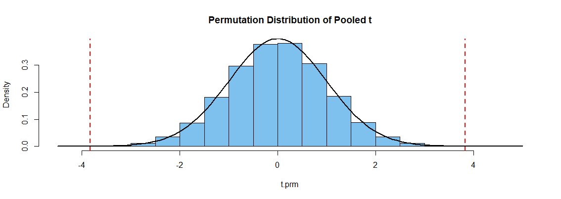
The figure below shows a histogram of the simulated permutation distribution. [It happens to match the density curve (black) of Student's t distribution with 118 degrees of freedom rather well, because data were simulated as normal with nearly equal SDs.] The P-value is the proportion of permuted t statistics outside the vertical dotted lines.

Note: My data were generated in R as follows:

set.seed(818)
x1 = round(rnorm(60, 107, 15), 1); x2 = round(rnorm(60, 100, 14), 1)

Answer 2

1. The t-test does not assume normality of the dependent variable; it assumes normality conditional on the predictor. (See this thread: Where does the misconception that Y must be normally distributed come from?). A simple way to condition on your grouping variable is to look at a histogram of the dependent variable, splitting the data on your grouping variable.

2. Normality tests, like the Shapiro-Wilk test, may not be that informative. Small deviations from normality may come up as significant (see this thread: Is normality testing 'essentially useless'?). However, given your small sample size, this probably is not an issue. Nonetheless, it does not really matter (practically speaking) if normality is violated, but the extent to which it is violated.

3. Depending on how non-normal your data might be, you probably do not have much to worry about. The general linear model (of which the t-test is a part) is more robust to violations of the normality assumption than to other assumptions (such as independence of observations). Just how robust it is has been discussed on this website before, such as in this thread: How robust is the independent samples t-test when the distributions of the samples are non-normal?. There are many papers looking at how robust this method is to violations of normality, as well (as evidenced by this quick Scholar search: https://scholar.google.com/scholar?hl=en&as_sdt=0%2C33&q=t-test+robust+to+nonnormality&btnG=).

4. You might as well run a nonparametric test and see if your conclusions differ; it costs essentially nothing to do so. The most popular alternative is the Mann-Whitney test, which is done with the stats::wilcox.test function in R (http://stat.ethz.ch/R-manual/R-devel/library/stats/html/wilcox.test.html). There are a lot of good introductions to this test on the internet—I would Google around until a description of it clicks with you. I find this video, calculating the test statistic by hand, to be very intuitive: https://www.youtube.com/watch?v=BT1FKd1Qzjw. Of course, you use a computer to calculate this, but I like knowing what's going on underneath.

Answer 3

One thing to keep in mind- outside of some contexts in physics, no process in nature will generate purely normally distributed data (or data with any particular nicely behaved distribution). What does this mean in practice? It means that if you possessed an omnipotent test for normality, the test would reject 100% of the time, because your data will essentially always only be, at best, approximately normal. This is why learning to ascertain the extent of approximate normality and its possible effects on inference is so important for researchers, rather than relying on tests.