2
$\begingroup$

I have the model

$$y=\beta_1 e^{\beta_2 x}+\beta_3 z+\epsilon$$

where $z$ is an indicator variable. I need to obtain estimates from linear regression to get initial values for the parameters. Then I can do an iterative search to find the best values for each parameter. However, I am having trouble doing this.

For the model

$$y=\beta_1 e^{\beta_2 x}+\epsilon$$

I can simply take the natural log of both sides and run the regression model

$$log(y)=log(\beta_1)+\beta_2 x+\epsilon$$

to get estimates of $\beta_1$ and $\beta_2$ but

$$y=\beta_1 e^{\beta_2 x}+\beta_3 z+\epsilon$$

doesn't appear to be intrinsically linear.

Any suggestions would be greatly appreciated.

Edit:

The data is as follows

df <- read.table(textConnection(
'x y z log_y
0.5 0.68 0  -0.38566
0.5 1.58 1  0.45742
1.0 0.45 0  -0.79851
1.0 2.66 1  0.97833
2.0 2.50 0  0.91629
2.0 2.04 1  0.71295
4.0 6.19 0  1.82294
4.0 7.85 1  2.06051
8.0 56.10 0 4.02714
8.0 54.20 1 3.99268
9.0 89.80 0 4.49758
9.0 90.20 1 4.50203
10.0 147.70 0 4.99518
10.0 146.30 1 4.98566'), header = TRUE)

When the model is just $y=\beta_1 e^{\beta_2 x}$ I get parameters estimates of 0.753 and 0.533 respectively after transforming the data to be linear. In SAS, I used these as the initial values for the new model and let $\beta_3=0$, arbitrarily. Using the Gaussian-Newton method, I got that the convergence criterion was met so it may be a valid approach. The coefficients I obtained in SAS are as follows:

enter image description here

$\endgroup$
22
  • 1
    $\begingroup$ Why do you need to creat initial values by linear regression, why don’t you use a reasonable values on the iterative nonlinear programming optimization? $\endgroup$
    – forecaster
    Commented Oct 6, 2018 at 3:09
  • $\begingroup$ That's how I was taught to do it. For the case where we have $log(y)=log(\beta_1)+\beta_2 x$ I got starting values of $.753$ and $.533$. I was thinking maybe to adapt for this model, I could use those same starting values and set $\beta_3 = 0$. SAS shows that this meets the convergence criterion so it may be a valid approach. $\endgroup$
    – Remy
    Commented Oct 6, 2018 at 3:17
  • 1
    $\begingroup$ Your use of logarithms is incorrect: $\log (a+b) \neq \log a + \log b$. $\endgroup$
    – Ben
    Commented Oct 6, 2018 at 9:07
  • $\begingroup$ I know that. I'm giving an example of a different model $y=\beta_1 e^{\beta_2 x}$ which is intrinsically linear. $\endgroup$
    – Remy
    Commented Oct 6, 2018 at 9:14
  • 1
    $\begingroup$ @Remy, (1) is the example data the real data of your problem or did you create it for this question? (2) what is your question, you ask for suggestion, but you do not explain your problem, what is wrong with your current solution? (3) Could you add the 'self-study' tag if this is a homework question. $\endgroup$ Commented Oct 8, 2018 at 12:14

2 Answers 2

1
$\begingroup$

I haven't read the whole comment thread, but this seems to work. I get the following estimates for the betas and $\sigma^2$: $1.1021399, 0.4884926 1.1266743, \exp(0.2739612)$. Notice that there are no linear approximations required (in the sense that you don't need to estimate a substitute model), and no derivatives required like there are in the Gaussian-Newton method.

df <- read.table(textConnection(
  'x y z log_y
0.5 0.68 0  -0.38566
0.5 1.58 1  0.45742
1.0 0.45 0  -0.79851
1.0 2.66 1  0.97833
2.0 2.50 0  0.91629
2.0 2.04 1  0.71295
4.0 6.19 0  1.82294
4.0 7.85 1  2.06051
8.0 56.10 0 4.02714
8.0 54.20 1 3.99268
9.0 89.80 0 4.49758
9.0 90.20 1 4.50203
10.0 147.70 0 4.99518
10.0 146.30 1 4.98566'), header = TRUE)


neg_log_like  <- function(params){
  beta1 <- params[1]; beta2 <- params[2]; beta3 <- params[3]; logSigmaSq <- params[4]
  meanVec <- beta1 * exp(beta2*df$x) + beta3*df$z
  sds <- rep(exp(logSigmaSq/2), length(meanVec))
  -sum(dnorm(df$y, meanVec, sds, log=T))
}

init_guess <- c(1,1,1,0.0)
optim(par = init_guess, 
      fn = neg_log_like,
      method = "Nelder-Mead")

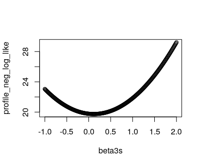
Edit: yes, thanks for pointing out the starting value issue. From the question it sounded more like a "how do I do this at all" issue. The log-likelihood is pretty flat in beta3, so you might consider taking this into account. Here's a plot of the profile negative log-likelihood using the other optimized values I obtained (not beta 3) using the following code

beta3s <- seq(-1, 2, .01)
profile_neg_log_like <- sapply(beta3s, function(beta3) neg_log_like(c(1.1021399, 0.4884926, beta3, 0.2739612)))
plot(beta3s, profile_neg_log_like)

enter image description here

$.2$ looks about right.

Also, notice that if you start off with $\beta_3$ at $0$, and scale up the $\beta_3$ values, you even get a negative estimate:

init_guess <- c(1,1,0,0.0)
res <- optim(par = init_guess, fn = neg_log_like,
             method = "Nelder-Mead", control = list(parscale=c(1, 1, 100, 1)))
cat(res$par)
#1.161925 0.4836862 -0.7783124 0.2670566
$\endgroup$
4
  • $\begingroup$ Interesting that your $\beta_1$ and $\beta_2$ are very close to mine but $\beta_3$ is significantly different. $\endgroup$
    – Remy
    Commented Oct 8, 2018 at 19:09
  • $\begingroup$ If by "linear approximation" you're referring to my comments or answers on another thread, then please be aware that the point is to find a good starting value for an iterative solution. You avoided this only by starting with an arbitrary guess of the solution--and you could do substantially better. Most black-box nonlinear optimizers require some reasonable starting value in order to work at all. Try $(1,1,0,0)$ for instance :-). @Remy as I indicated in a comment to your question, estimate $\beta_3$ as the mean difference in responses between the two groups. You'll get about 0.2. $\endgroup$
    – whuber
    Commented Oct 8, 2018 at 19:14
  • $\begingroup$ @whuber Right, that is what I have used as my initial value for $\beta_3$. But would I be correct in estimating $\beta_1$ and $\beta_2$ by modeling $\text{log}(y-0.2014)=\text{log}(\beta_1)+\beta_2 x$ $\endgroup$
    – Remy
    Commented Oct 8, 2018 at 19:21
  • 1
    $\begingroup$ It's the right idea, but you have to be careful not to take logs of negative values. Here's some code based on that other thread. It converges in 6 iterations and gives you p-values for all parameters, too: b.3 <- mean(subset(df, z==1)$y) - mean(subset(df, z==0)$y); c.0 <- 0.5 * min(df$y - df$z*b.3); model.0 <- lm(log(y - c.0 - z*b.3) ~ x, df); b.1 <- exp(coef(model.0)["(Intercept)"]); b.2 <- coef(model.0)["x"]; start <- list(b.1=b.1, b.2=b.2, b.3=b.3); model <- nls(y ~ b.1 * exp(b.2 * x) + b.3*z, data = df, start = start); summary(model) $\endgroup$
    – whuber
    Commented Oct 8, 2018 at 22:08
0
$\begingroup$

This needs to be fit like a non-linear regression. You can do it with a ML estimate as proposed by Taylor, or you can use Bayesian MCMC sampling. My estimate using MCMC sampling in JAGS is very similar to your results:

            Mean          SD   P.value       2.5%     97.5% Time-series SE     psrf  psrf CI
b[1]   1.0700276 0.069644097 0.000 ***  0.9413769 1.2183012   0.0029073561 1.006867 1.024380
b[2]   0.4926133 0.006674661 0.000 ***  0.4790468 0.5055502   0.0002762362 1.006998 1.024800
b[3]  -0.1291385 0.490887669 0.388     -1.1131594 0.8441626   0.0080573350 1.001177 1.004308
sigma  1.0310585 0.264173711 0.000 ***  0.6631381 1.6864203   0.0035488911 1.000404 1.000565

The code is here:

df <- read.table(textConnection(
'x y z log_y
0.5 0.68 0  -0.38566
0.5 1.58 1  0.45742
1.0 0.45 0  -0.79851
1.0 2.66 1  0.97833
2.0 2.50 0  0.91629
2.0 2.04 1  0.71295
4.0 6.19 0  1.82294
4.0 7.85 1  2.06051
8.0 56.10 0 4.02714
8.0 54.20 1 3.99268
9.0 89.80 0 4.49758
9.0 90.20 1 4.50203
10.0 147.70 0 4.99518
10.0 146.30 1 4.98566'), header = TRUE)

require(runjags)

do_DIC <- FALSE
fast_model_run <- FALSE
jags_parallel <- FALSE

##########

repeat {

model_file <- paste0(tempdir(), "/tmp_bugs_model.txt")
sink(model_file)
cat("model {

sigma ~ dunif(0, 10)
b[1] ~ dnorm(0, 0.01)
b[2] ~ dnorm(0, 0.01)
b[3] ~ dnorm(0, 0.01)

for (i in 1:n) {
    y_exp[i] <- b[1]*exp(b[2]*x[i]) + b[3]*z[i]
    y[i] ~ dnorm(y_exp[i], 1/sigma^2)
}

}
")
sink()


win.data <- c(df, n = nrow(df))


inits <- function () { 
list(
    b = rnorm(3, 0, 1)
) 
}

params = c("b", "sigma")
if (do_DIC)
    params <- c(params, "dic", "ped") 

#
if (fast_model_run) { # pro porovnavani casu (vic chainu -> stabilnejsi)
ni <- 20000
nt <- 1
nb <- 10000
nc <- 3
adapt <- 0
} else if (1) { # FINALNI pro paper
# ni: 1000 -> .. sec
ni <- 20000
nt <- 10
nb <- 10000
nc <- 3
adapt <- 5000
} else { # klasicky run
ni <- 1000
nt <- 1
nb <- 500
nc <- 3
adapt <- 0
}


# runjags package

#if (!exists("model_info"))
    model_info <- list()

start_time <- Sys.time()
print(start_time)
t1 <- proc.time()
outRJ <- run.jags(model_file, params, win.data, nc, inits, 
    method = ifelse(jags_parallel, "rjparallel", runjags.getOption("method")),
    keep.jags.files = FALSE,
      nb * nt, ni - nb, thin = nt, summarise=FALSE, adapt = adapt, modules = "glm",
    silent.jags = !isatty(stdout())) # adapt = 0
        # pri presmerovani do filu nechceme progress bar
t2 <- proc.time()
print(t2 - t1)
end_time <- Sys.time()
print(end_time)

break

}

par(ask = TRUE)
plot(outRJ$mcmc)
s1 <- mcmcsum(outRJ$mcmc)
$\endgroup$

Not the answer you're looking for? Browse other questions tagged or ask your own question.