Finding Initial Parameter Values for Gompertz Model with Intercept

Question

I have the following data:

y x
1275 230
1350 235
1650 250
2000 277
3750 522
4222 545
5018 625
6125 713
6200 735
8150 820
9975 992
12200 1322
12750 1900
13014 2022
13275 2155

I would like to find reasonable initial values for the model

$$y=\alpha+\beta_1\text{exp}(-\beta_2 e^{-\beta_3 x})+\epsilon$$

What I know:

For the Gompertz model, the inflection point satisfies

$$x=\frac{\text{log}(\beta_2)}{\beta_3}$$

For the Gompertz model we have

$$\lim_{x\rightarrow\infty} \beta_1\text{exp}(-\beta_2 e^{-\beta_3 x})=\beta_1$$

so presumably with an intercept we have

$$\lim_{x\rightarrow\infty} \alpha+\beta_1\text{exp}(-\beta_2 e^{-\beta_3 x})=\alpha+\beta_1$$

so we can set $\alpha+\beta_1=13275$, the maximum value of $y$ in the dataset.

However, I can't seem to combine what I know to find initial values.

I would like to find reasonable initial values and not rely on specifying an exhaustive grid of values.

Any ideas or suggestions would be appreciated.

Update:

I read on wikipedia that the halfway point is found to be

$${\displaystyle x_{\text{hwp}}=-{\frac {\ln\left(\frac{ln(2)}{\beta_2}\right)}{\beta_3}}}$$

I let $x_{\text{hwp}}=713$, the median of the $x$'s.

As previously stated, I have $$x=\frac{\text{log}(\beta_2)}{\beta_3}$$

I let $x=1000$, since a plot of the data shows that a possible inflection point is around there.

By software, this system of equation results in $\beta_2=0.279$ and $\beta_3=-0.0013$.

I (randomly) decided to let $\alpha=13275$ and $\beta_1=-13275$, where $13275$ is the maximum value of $y$.

The model then converges after 15 iterations to

$$\hat{y}=12934.4-14349.2\cdot\text{exp}(-0.1214e^{0.00257x})$$

which are reasonably close to my initial estimates. I'm not sure why it would make sense to have $\hat{\alpha}=13275$ and $\hat{\beta_1}=-13275$ though.

Answer 1

A typical situation in nonlinear statistical modeling is that the at least some of the parameters of interest to the modeler are not good parameters to use for parameterizing the model. I have found that is really difficult to convince a lot of people that they should parameterize their model in terms of parameters in which they have no interest. Well duh! It often turns out to be a good idea, however, because these new parameters lead to an easier and more stable estimation scheme. Once these uninteresting parameters have been estimated the parameters of interest can be calculated from them. This is how it goes.

step1: rescale the problem so that $x(15)=1$ and $y(15)=1$ this is just standard good advice for any model when it is possible.

step2: replace the independent variables $\alpha$ and $\beta_1$ with new independent variables $y_1$ and $y_n$. Note that these are parameters and not observations. They are the predicted observed $y$ values for $x(1)$ and $x(15)$. However we have very good initial estimates for them namely the observed values $y(1)$ and $y(n)$ for the values $x(1)$ and $x(n)$. Now since you have rescaled the $y$'s a good initial value for $y_n$ is 1.0 for $y_1$ it is 0.096045. You can use almost any reasonable starting values for $\beta_2$ and $\beta_3$, but they both should be $>0$, say $\beta_2=0.1$, $\beta_3=0.1$ It is not at all sensitive to these initial values. The initial values $\beta_2=10$, $\beta_3=10$ converge to the same solution.

step 3: Solve the linear system

\begin{align} y_1&=\alpha+\beta_1\text{exp}(-\beta_2 e^{-\beta_3 x(1)}) \\ y_n&=\alpha+\beta_1\text{exp}(-\beta_2 e^{-\beta_3 }) \\ \end{align}

for $\alpha$ and $\beta_1$ in terms of $y_1,y_n,\beta_2,$ and $\beta_3$ This is just a little bit of matrix algebra. In any system which supports matrix algebra. You form the matrix $M$ $$ M= \begin{bmatrix} 1&\exp(-\beta_2 e^{-\beta_3 x(1)}) \\ 1&\exp(-\beta_2 e^{-\beta_3})\ \ \\ \end{bmatrix} $$ Then $$ \begin{bmatrix} \alpha \\ \beta_1 \\ \end{bmatrix} = M^{-1} \begin{bmatrix} y_1 \\ y_n \\ \end{bmatrix} $$

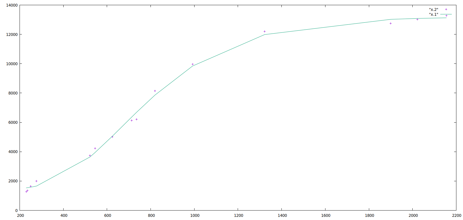
Now the minimization is carried out in two phases. For the first phase $\beta_2$ and $\beta_3$ are estimated for the fixed values of $y_1$ and $y_n$. In the second phase all four parameters are estimated. Hereis the fitted data plot.

The estimates for the original parameters are 1403.9062 11799.399 9.8326183 0.0034059501 Notice that at no time did one need to look at any aspect of the data. The only assumption involved is that a Gompertz curve should be used. Everything else is automatic. This same procedure works for many kinds of growth curves. I used AD Model Builder to fit the model, but it can easily be done in R (so it must be simple).