Is there a skewed probability density function that models a normal distribution with two parameters, $σ_1$ and $σ_2$?

Question

Is there a way to model data that are skew normally distributed, but for which one builds in two seperate standard deviations?

The parameter $σ_1$ should specify the 15.9% to 50% interval, whereas $σ_2$ should specify the 50% to 84.1% interval (i.e., the middle 68.2% of values).

The idea is that the values of $σ_1$ and $σ_2$ should be computed from the data; and together with the mean, give parameters to plot the representative probability density function. The result will look skew normally distributed, unless $σ_1 = σ_2$, in which case the PDF would be modeled as a normal curve. Importantly, the area under the probability density curve between $σ_1$ and the mean as well as the area between the mean and $σ_2$ should both be 34.1% of the probability and 68.2% when combined.

Note that the skew normal distribution, the log-normal distribution and the Raleigh distribution does not seem to allow this trivially as they don't have two such $σ_1$ and $σ_2$ parameters.

An example for which $σ_2 > σ_1$:

Answer 1

There is an elegant solution to this problem.

We'll calculate two normal curves, let's call them the lower curve and the higher curve (referring to lower and higher values of the dependent variable, viz. the left and right from the mean).

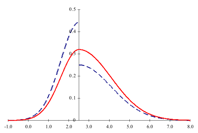
As mentioned in the question, we have from the data parameters $σ_1$ and $σ_2$ that specify the 15.9% to 50% interval and the 50% to 84.1% interval, respectively. Now, we calculate the two normal distributions centered at the mean. For the upper curve, we use $σ_2$ and we remove its lower half. For the lower curve, we use $σ_1$ and we remove its upper half. This give us the dashed lines:

Then, the red solid line is the result of scaling the upper and the lower curve so that they meet at the mean.

You'll notice that we use the mean, and not the mode. The reason for this is that we care about the area of the curve, not the discrete frequencies. In fact, although it is only alluded to in the question, the use case for this question is in fact cumulative time series data.

This, however, invites the question: Since we have scaled, we also lose the 15.9% -> 50% -> 84.1% rule, and hence this breaks the requirement in the posted question. This leads us to the final modification.

There may be other (better) ways to modify the now continuous curve to spread the probability density back to the required 15.9% -> 50% -> 84.1% rule. However, probably the peak of the curve will have to be moved.

My suggestion is then to move the peak of the curve to the lower position (viz. to the left) so that at the mean point the cumulative density is restored to 50%. Note that if $σ_1 > σ_2$, one has to move the curve to the upper position instead, since then the curve is then left-skewed.

After this final modification, the curve retains the 50%-50% split about the mean, with a form that roughly matches the data; having been constructed from the halves of the two normal curves with sd's $σ_1$ and $σ_2$, respectively. Although the means are the same, the peak is shifted in the final step to distribute each 50% of the density correctly.

Pic Source: The Two-Piece Normal, Binormal, or Double Gaussian Distribution: Its Origin and Rediscoveries (by Kenneth F. Wallis).