Sample from aggregate portfolio distribution versus individual asset distributions

Question

Suppose I have three assets $x_1,x_2,x_3$ in a portfolio with weights $W=\begin{bmatrix} w_1 \\ w_2 \\ w_3 \end{bmatrix} $, expected returns $R=\begin{bmatrix} \mu_1 \\ \mu_2 \\ \mu_3 \end{bmatrix}$, and a covariance matrix $V$.

The expected return of my portfolio is $\mu_p=W^TR$ and the variance of my portfolio is $\sigma^2_p=W^TVW$.

I would like to run Monte Carlo simulations on my portfolio using a normal distribution.

I can do this either by:

1. Sampling from the distribution of portfolio returns $N(\mu_p,\sigma^2_p)$.
2. Sample from the three individual asset returns and use those three returns to compute my overall portfolio return.

First, how would I accomplish the second approach (would I be sampling from a multivariate normal distribution)?

Second, are these two approaches equivalent as long as I assume that the weights $W$ of my portfolio remain the same?

Answer 1

First, how would I accomplish the second approach (would I be sampling from a multivariate normal distribution)?

You can indeed do this by sampling from a multivariate normal distribution. If you are using R for your simulations then you can sample using the mvrnorm function in the MASS package. Here is an example where I have generated a large number of simulated values using a given mean vector and variance matrix:

set.seed(1);

#Create example of mean vector and variance matrix
#Checked eigenvalues to ensure it is a valid variance matrix
M <- matrix(c(16, 17, 14), ncol = 1);
V <- matrix(c(3.2, 1.1, 1.5, 1.1, 4.8, 2.1, 1.5, 2.1, 6.0), ncol = 3);

#Generate n values from normal distribution with above mean and variance
library(MASS);
n    <- 10^5;
SIM1 <- mvrnorm(n, mu = M, Sigma = V);

Alternatively, you can also generate independent standard normal random variables and transform them so that they come from the desired multivariate normal distribution:

#Find principal square root of variance matrix
SS  <- diag(eigen(V)$value);
EE  <- eigen(V)$vectors;
S   <- EE %*% sqrt(SS) %*% t(EE);

#Generate n values from normal distribution with above mean and variance
SIMB <- matrix(0, nrow = n, ncol = 3);
for (i in 1:n) { SIMB[i,] <- t(M + S %*% rnorm(3,0,1)); }

---

Second, are these two approaches equivalent as long as I assume that the weights W of my portfolio remain the same?

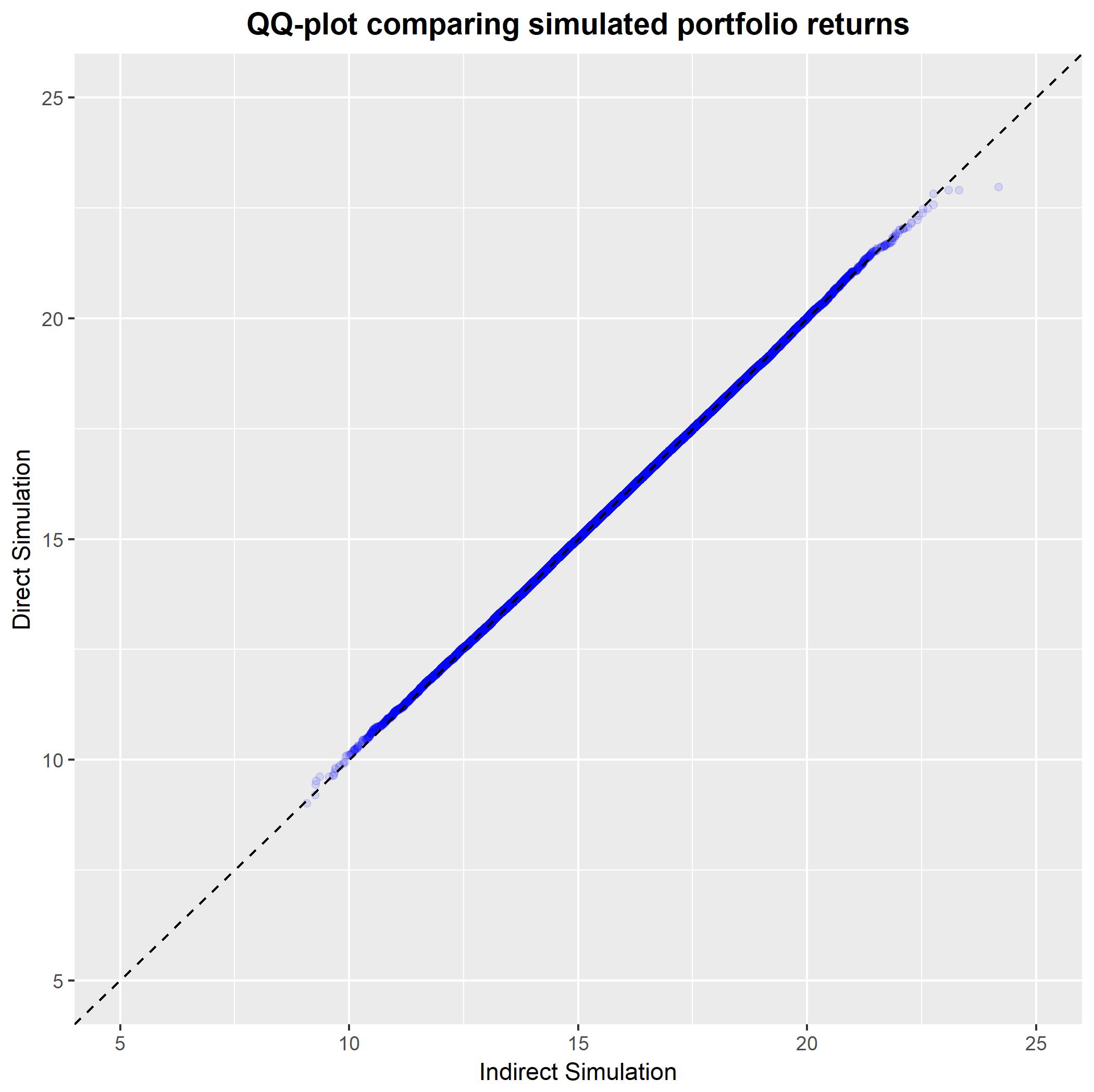
Yes, they are the same. Your derivation of the distribution of your portfolio return is correct, and so the two simulations should yield values from the same distribution. To confirm this, let's go ahead and simulate using the direct method and then generate a QQ-plot to confirm that both methods give values from the same distribution:

#Create example weights
W <- c(0.2, 0.5, 0.3);

#Generate values for portfolio return via indirect method
VALS1 <- rep(0, n);
for (i in 1:n) { VALS1[i] <- sum(W*SIM1[i,]) }

#Generate values for portfolio return via direct method
MP    <- sum(W*M);
VP    <- t(W) %*% V %*% W;
VALS2 <- rnorm(n, mean = MP, sd = sqrt(VP));

#Create QQ-plot comparing values
plot(sort(VALS1), sort(VALS2), 
     main = 'QQ-plot comparing simulated portfolio returns',
     xlab = 'Indirect Simulation', ylab = 'Direct Simulation');
abline(a = 0, b = 1, lty = 3);

ggplot(data = data.frame(x = sort(VALS1), y = sort(VALS2)),
       aes(x = x, y = y)) +
geom_point(alpha = 0.1, colour = 'blue') +
geom_abline(intercept = 0, slope = 1, linetype = 'dashed') +
scale_x_continuous(limits = c(5,25)) +
scale_y_continuous(limits = c(5,25)) +
theme(plot.title    = element_text(hjust = 0.5, size = 14, face = 'bold')) +
ggtitle('QQ-plot comparing simulated portfolio returns') +
xlab('Indirect Simulation') + ylab('Direct Simulation');