Failing to implement Bayesian Chi2 goodness of fit test

Question

I am trying to implement one of the methods described in Valen Johnson's A Bayesian Chi-Squared Test for Goodness of Fit. It presents a couple of variants depending on whether the random variable of interest is continuous or discrete but I am specifically interested in a binomial outcome.

The central idea is that the proposed $R^B$ statistic's posterior approaches a $\chi^2_{K-1}$ distribution, where $K$ is the number of discrete values a variable can take. It is defined as

$$R^B(\tilde\theta) = \sum_{k=1}^K \left[{m_k - n p_k(\tilde\theta) \over \sqrt{np_k(\tilde\theta)}}\right]^2$$

where $\tilde\theta$ is a single posterior draw from the parameter vector, $p_k$ is the expected count, calculated over the $n$ observations as

$$p_k(\tilde\theta) = {1 \over n}\sum_{j=1}^n \sum_{y \in \text{bin} k} f_j(y\mid\tilde\theta).$$

The above notation is directly transcribed from the paper, but the notion of bins is irrelevant for my binomial scenario, so a slightly clearer way of denoting this is

$$p_k(\tilde\theta) = {1 \over n}\sum_{j=1}^n f(k -1\mid\tilde\theta_j),$$

since there's only one possible $y$ value at each level $k$ and counting starts at $0$. Also, I shifted the $j$ subindex from the pmf $f$ to the parameter $\tilde\theta$, as the pmf has a fixed functional form, but parameters can be observation-dependent (e.g. the mean in a regression model).

Finally, we have $m_k$, which corresponds to observed counts. Using $I(.)$ to denote the indicator function and $a_k$ for the corresponding quantile, we have

$$m_k(\tilde\theta)=\sum_{j=1}^n I(F(y_j\mid\tilde\theta_j) \in (a_{k-1}, a_k]).$$

For reference, the equations above are numbered $(2)$ through $(5)$ in the paper.

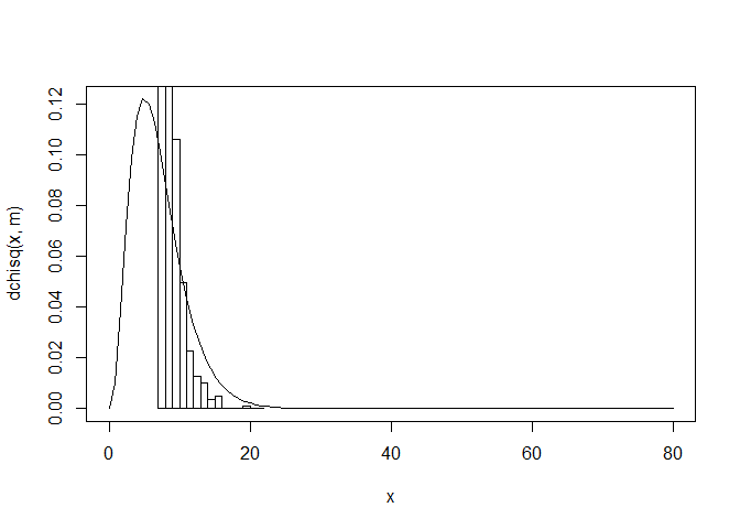
Having implemented this measure for a simple intercept-only logistic regression model in R, the distribution is far from what the paper says it should look like. Here's the code:

library(rstanarm)
library(dplyr)

# Calculate R^B statistic for single posterior draw
iRB <- function(b, n, data) {

  y <- data*n
  p <- (1/(1+exp(-rep(b, length(y)))))

  pmf <- function(X) dbinom(X, n, p)
  cdf <- function(X) pbinom(X, n, p)

  rbk <- lapply(1:(n+1), function(k) {
      # eq (5)
    pk <- sum(pmf(k-1))
      # eq (4)
    Fy <- cdf(y)
      # eq (2)
    ak <- cdf(k-1.1);aK <- cdf(k-1)
    mk <- sum(ifelse(ak <Fy&Fy<= aK, 1, 0))

    data.frame(pk = pk, mk = mk)
    }) %>% do.call(rbind, .)

  with(rbk,sum(((mk - pk)/sqrt(pk))**2))
}

# Simulate data
m <- 7
set.seed(1);binomdat <- data.frame(y=rbinom(100, m, 0.5)/m, m  = m)
# Fit intercept-only logistic regression
binomfit <- stan_glm(y ~ 1, family=binomial(), data=binomdat, weights = m)
# Extract posterior
ps <- as.matrix(binomfit)
# Calculate R^B for each posterior draw
chi2b <- sapply(ps, iRB, m, binomdat$y)

# Check results
curve(dchisq(x, m), from = 0, to = 80)
hist(chi2b, probability = T, add = T)

I've already gone over this with a professor and we're both perplexed by the results. Not sure if we're misreading the paper or overlooking an error in the implementation.

Answer 1

• The value/distribution that you have been calculating is the posterior distribution of $R^B$ (based on the posterior distribution of the parameter $\theta$ determined from a single sample/test $y$) but this is not chi-square distributed.

  When $n$ grows the posterior distribution for $\theta$ will approach some degenerate distribution around the true parameter value, and $R^B$ will be as well a degenerate distribution for a fixed value/sample/test $y$. This is like the sharp peak that you observe in your histogram, it is the chi-square statistic for a single sample/draw $y$, where you wiggle a little bit the predicted value $\theta$.

• The theorem 1 from the article relates to $R^B$ as a frequentist concept. It is the sample distribution of $R^B$ (based on multiple samples/tests $y$) which is chi-square distributed.

  E.g. if you do the test many times and take a single posterior sample $\tilde{\theta}$, for each test, from which you calculate $R^B(\tilde{\theta})$, then you will have $R^B \xrightarrow[\text{}]{\text{d}} \chi^2_{K-1}$.

---

#do this N times
N <- 500
chi2b <- rep(0,N)

pb <- txtProgressBar(title = "progress bar", min = 0,
                     max = N, style=3)
for (ii in 1:N) {
  binomdat <- data.frame(y=rbinom(100, m, 0.5)/m, m  = m)
  # Fit intercept-only logistic regression  # refresh = 0 suppresses output
  binomfit <- stan_glm(y ~ 1, family=binomial(), data=binomdat, weights = m, refresh= 0)
  # Extract SINGLE posterior
  ps <- as.matrix(binomfit)[1]
  # Calculate R^B for each posterior draw
  chi2b[ii] <- sapply(ps, iRB, m, binomdat$y)
  setTxtProgressBar(pb, ii)
}
close(pb)

# Check results
curve(dchisq(x, m), from = 0, to = 80)
hist(chi2b, probability = T, add = T, breaks = seq(0,80,1))