2
$\begingroup$

I am currently trying to fit a polynomial model to measurement data using the lm() function.

fit_poly4 <- lm(y ~ poly(x, degree = 4, raw = T), weights = w)

with x as independent,

y as dependent variable

and w = 1/variance of the measurements

summary(fit_poly4)

Call:
lm(formula = y ~ poly(x, degree = 4, raw = T), weights = w)

Weighted Residuals:
     Min       1Q   Median       3Q      Max 
-1.57259 -1.02934  0.00252  0.98814  1.48758 

Coefficients:
                                Estimate Std. Error t value Pr(>|t|)    
(Intercept)                      39.0375     3.4460  11.328 2.94e-13 ***
poly(x, degree = 4, raw = T)1  55.6996    17.7858   3.132 0.003501 ** 
poly(x, degree = 4, raw = T)2 -71.8194    19.9575  -3.599 0.000979 ***
poly(x, degree = 4, raw = T)3  23.8642     7.0456   3.387 0.001759 ** 
poly(x, degree = 4, raw = T)4  -2.4069     0.7507  -3.206 0.002872 ** 
---
Signif. codes:  0 ‘***’ 0.001 ‘**’ 0.01 ‘*’ 0.05 ‘.’ 0.1 ‘ ’ 1

Residual standard error: 1.069 on 35 degrees of freedom
Multiple R-squared:  0.8903,    Adjusted R-squared:  0.8778 
F-statistic: 71.04 on 4 and 35 DF,  p-value: 2.637e-16

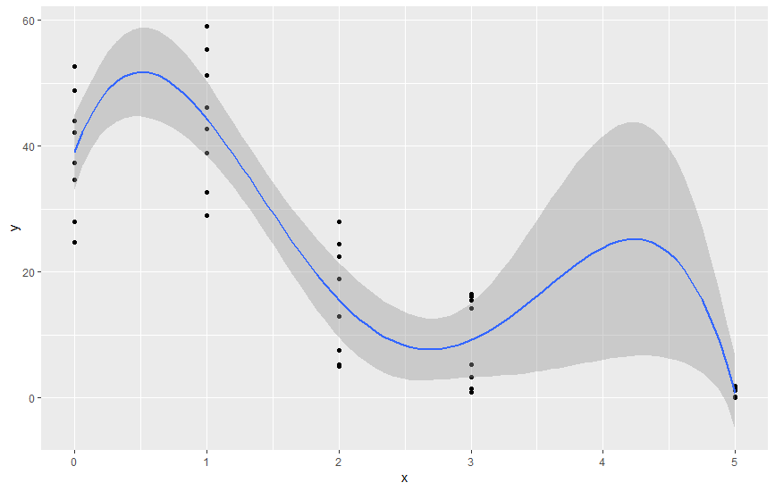
While this gives me nice enough results on the statistical side, the derived polynomial

y = 39.0375 + 55.6996*x - 71.8194*x^2 + 23.8642*x^3 - 2.4069*x^4

specifically the second peak between 3 and 5 (see picture) does not make sense for my specific case.

enter image description here

Therefore I want to try and use a given polynomial formula

y = -3,3583*x^4 + 43*x^3 - 191,14*x^2 + 328,2*x - 137,7

in lm().

I tried

fit_poly4 <- lm(y ~ 328.2*x-191.14*I(x^2)+43*I(x^3)-3.3583*I(x^4)-137.3, weights = w)

which just returns

Error in terms.formula(formula, data = data) : 
  invalid model formula in ExtractVars

How do I need to write my polynomial in lm() to get this to work?

Alternatively is there any way to force lm() to not produce a second peak but to smoothly decrease from 3 to 5?

I appreciate your help in advance, thank you.

Edit: The data represents biomass (y) over different vol% nutrient concentrations (x) and should be continuous.

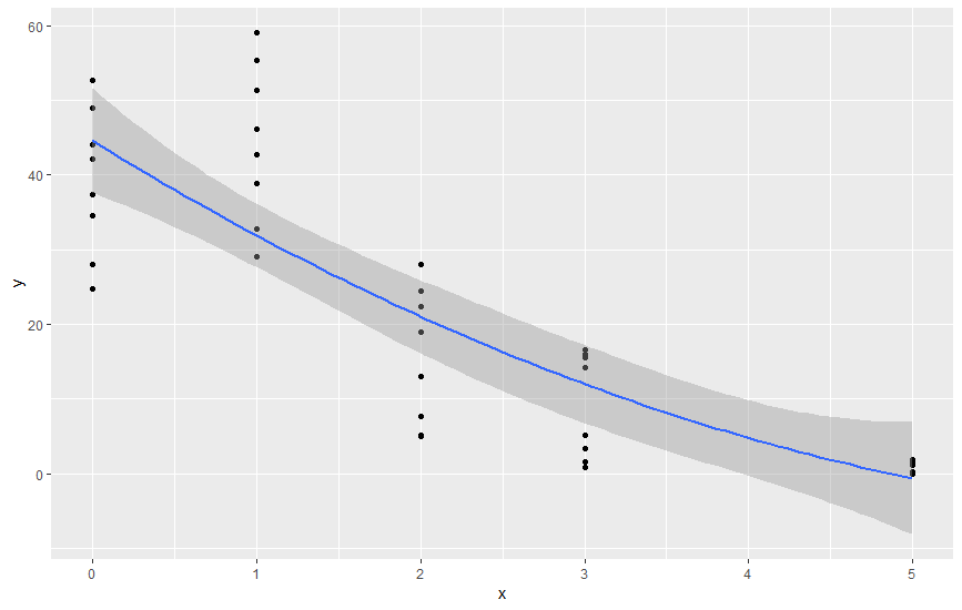
I've also tested simpler polynomials which either come back to imprecise in case of degree = 2

enter image description here

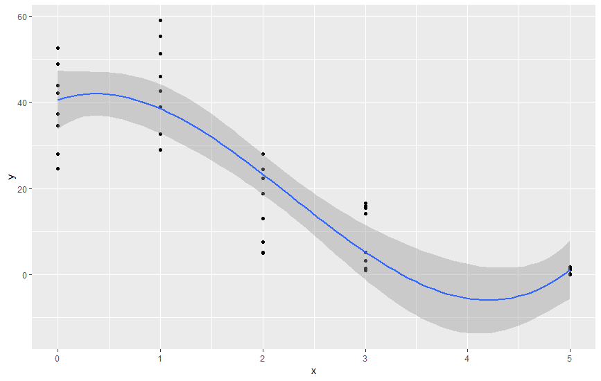
or have their own flaws (negative biomass) in case of degree = 3

enter image description here

$\endgroup$
2
  • 2
    $\begingroup$ Polynomials are not a good choice if you're trying to fit a smooth curve through discrete sets of x-values. You might consider (for example) natural regression splines with a few prespecified knots, or perhaps smoothing splines (or a variety of other options. Another possibility would be to use orthogonal polynomials with fairly strong regularization on the higher order terms, such as ridge regression or perhaps elastic net. At the very least you would need to impose the more obvious constraints on it. $\endgroup$
    – Glen_b
    Commented Apr 1, 2019 at 0:25
  • $\begingroup$ fitting on a log-y scale will take care of the possibility of negative predictions (also deal with some heteroscedasticity). Can we have a reproducible example? (I answered the technical question here, but it looks like there's room for some statistical questions as well ... $\endgroup$
    – Ben Bolker
    Commented Apr 1, 2019 at 0:38

1 Answer 1

1
$\begingroup$

That final peak is due to overfitting. Your model is way too complex for the data you are trying to fit. It is just finding the degree-4 polynomial that intersects the x value you have at the mean of its observations.

Is x a discrete variable? Because in that case, maybe this is not the right approach at all.

In other case, please consider a simpler polynomial fit

$\endgroup$
2
  • $\begingroup$ Thank you very much for your response. The data represents measured biomass over different vol% concentrations of nutrients and should therefore be continuous. I've also tested simpler polynomials (degree 2 and 3) which I also compared via anova() to eachother. The differences between the models always came back significant. $\endgroup$
    – MB93
    Commented Mar 31, 2019 at 19:31
  • 1
    $\begingroup$ I suggest a test where you average the Y values for each X, and then fit those five data points. In effect, this is what the regression software is doing so you should see similarly shaped curves. $\endgroup$ Commented Mar 31, 2019 at 21:26

Your Answer

By clicking “Post Your Answer”, you agree to our terms of service and acknowledge you have read our privacy policy.

Not the answer you're looking for? Browse other questions tagged or ask your own question.