Modelling rnbinom not returning pre-set parameters

Question

I am working with the rnbinom function in R but I think I have misunderstood the meaning of the parameters that get stipulated in the arguments.

For reference, I have been looking at the documentation here: https://stat.ethz.ch/R-manual/R-devel/library/stats/html/NegBinomial.html

I have generated a random vector like so:

z <- rnbinom(500000, 0.16, 0.19)

My understanding is that I have called for 500000 random values from a negative binomial distribution with a dispersion (theta) parameter of 0.16. For the prob argument I entered 0.19, which is defined as "probability of success in each trial. 0 < prob <= 1." I have interpreted this argument as setting an "effect size" that would be returned if the simulated data is fit back into a negative binomial regression model. However, my understanding is evidently wrong. Please see the below for a step-by-step.

---

Load libraries

library(ggplot2)
library(reshape2)
library(MASS)

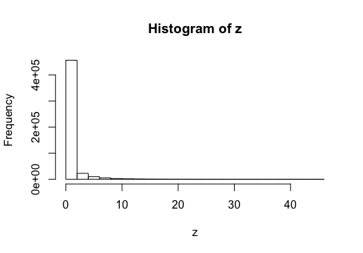
When I plot the vector it looks like this:

hist(z)

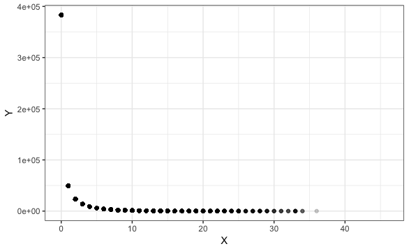
Based on this histogram, the randomly generated vector is then transformed into a 2-column dataframe where the original values act as Xs and the frequencies act as Ys, like so:

dat <- data.frame(z=z,freq=as.vector(table(z)[as.character(z)]))

Rename columns:

colnames(dat) <- c("X","Y")

Plotting this X-Y dataframe looks like this:

g1 <- ggplot(dat, aes(x = z, y = freq))+
  geom_point(alpha = .2)+
  theme_bw()+
  labs(x = "X", y = "Y")
g1

Then, I attempt to fit this dataframe back into a negative binomial regression model:

M0 <- glm.nb(Y ~ X, data = dat)
summary(M0)

But I get this error:

Error: no valid set of coefficients has been found: please supply starting values
In addition: Warning message:
glm.fit: fitted rates numerically 0 occurred 

What is happening here? I had expected the model to return a regression coefficient of 0.19 as I stipulated in the original random vector generation.

Answer 1

I am unclear why you believe you need to supply dat to glm.nb(). The easiest way of setting up a model with no predictors would be simply

> model <- glm.nb(z~1)

We can now inspect it:

> coef(model)
(Intercept) 
 -0.3807305 
> model$theta
[1] 0.160006

So the theta output matches the 0.16 you put in. What does the estimated intercept of -0.3807 have to do with your 0.19?

First, note that we did not give the link parameter to glm.nb(), so it used the default link function, which is the log.

> exp(coef(model))
(Intercept) 
   0.683362 

Second, note that glm.nb() uses a particular one of the many, many parameterizations of the negbin distribution (I recommend Hilbe's Negative Binomial Regression). Specifically, it models the mean (on the log scale). Let's verify:

> mean(z)
[1] 0.683362

This looks good.

So, how do we recover your 0.19? Since you didn't name the parameters you gave to rnbinom(), it by default fed your arguments 500000, 0.16, 0.19 into its first three parameters: n=500000, size=0.16, prob=0.19. A look at ?rnbinom tells us that the mean of your random numbers should be size*(1-prob)/prob. Let's check:

> size <- 0.16
> prob <- 0.19
> size*(1-prob)/prob
[1] 0.6821053

This again looks good. So all we have to do is to solve this equation for the mean which glm.nb() fitted (on a log scale) to recover your prob parameter:

> model$theta/(exp(coef(model))+model$theta)
(Intercept) 
  0.1889737