4
$\begingroup$

I'm taking a data camp lesson by Professor Rob J Hyndman. He went over the ACF plot and said that you know the period of seasonality based on the highest point in the ACF plot.

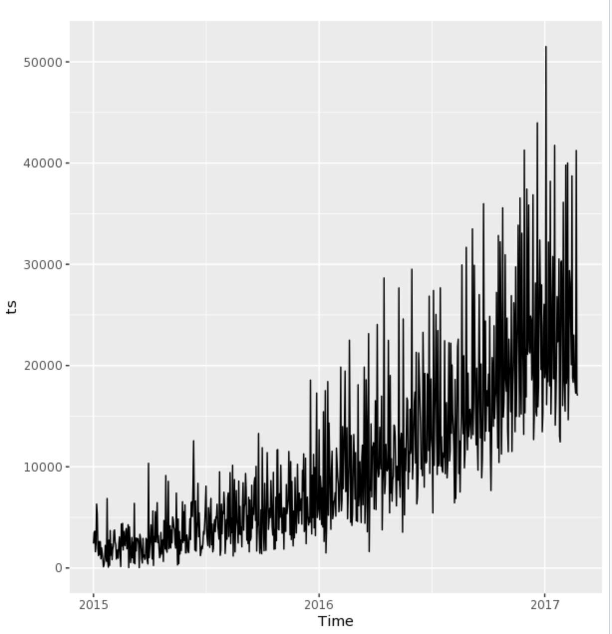
I have this timeseries-

enter image description here

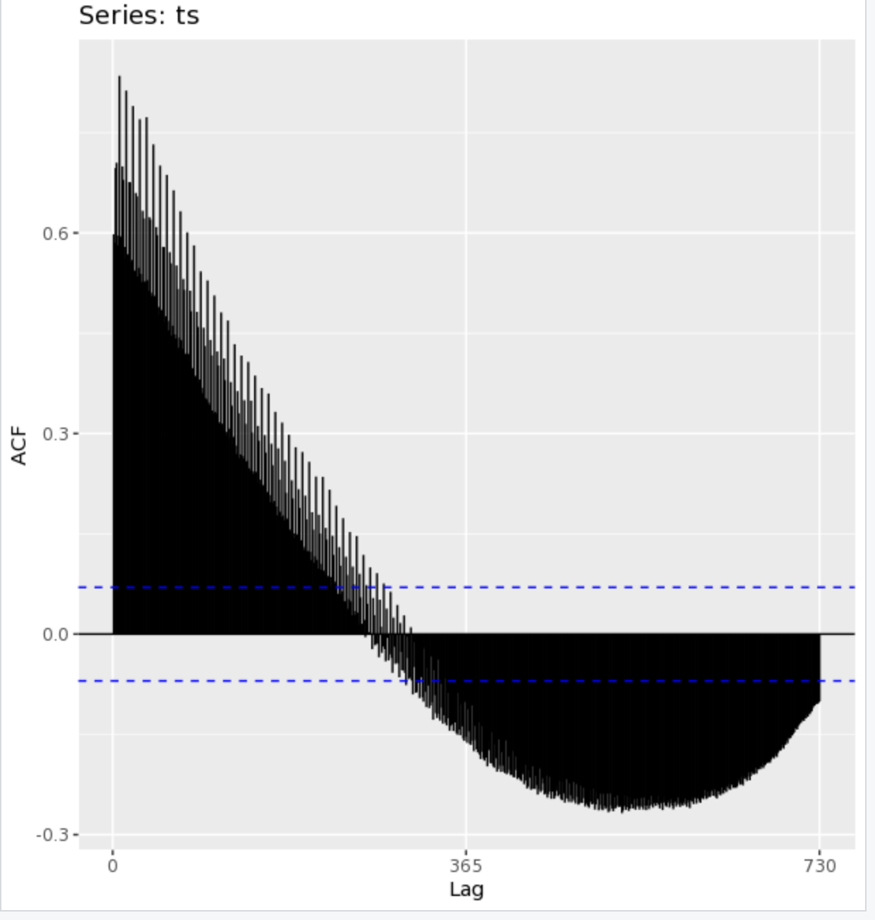
And I have this ACF plot -

enter image description here

Does this mean the seasonal difference is every one or two days and the further out in time, the more strongly negatively correlated the relationship? I'm not sure how to read it with this many significant lags.

Update-

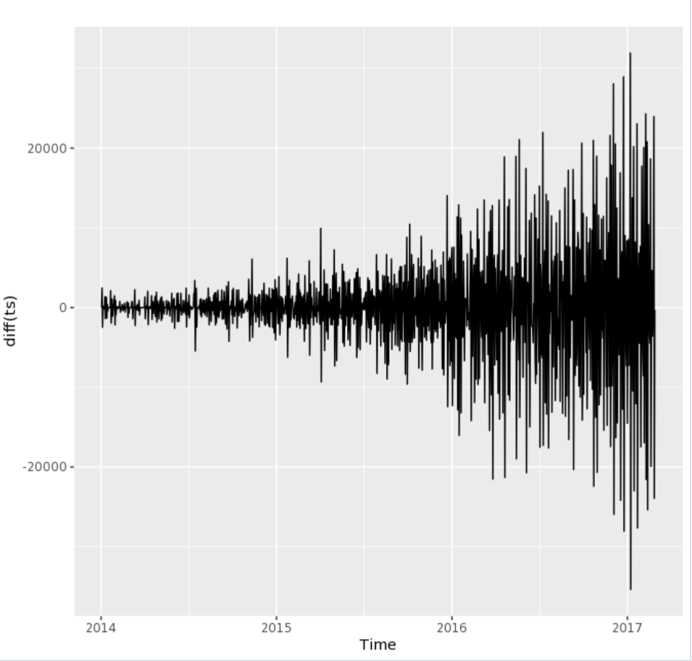
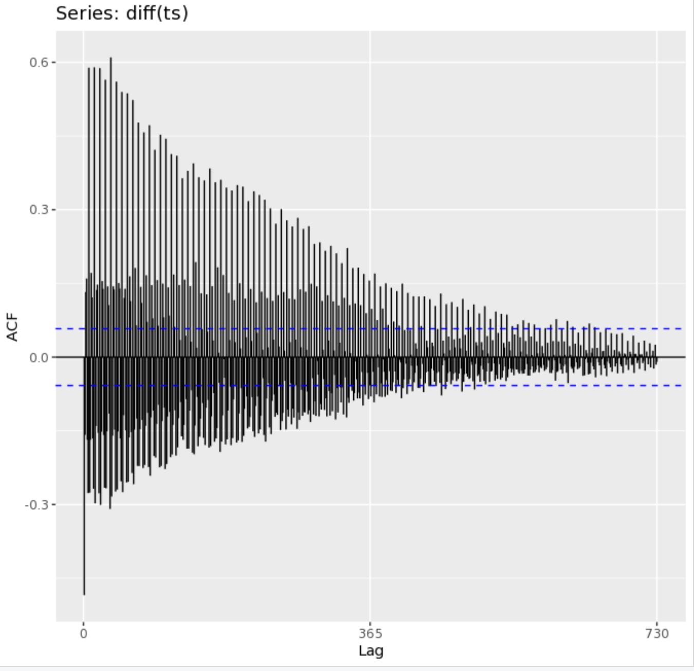
I created an arima model with auto.arima() and it suggested that I diff my timeseries one time to make it stationary. I'll add the new charts.

Autoplot on the stationary data-

enter image description here

ACF of the stationary data-

enter image description here

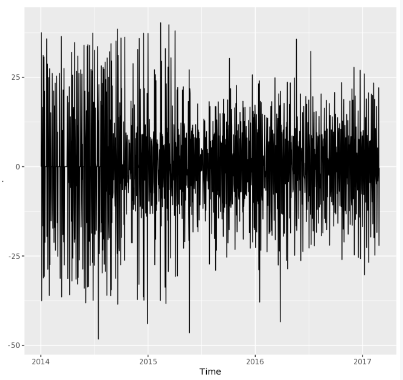
I added a transformation for the increasing variance.

ts %>% BoxCox(lambda = .3170305) %>% diff() %>% autoplot() where lambda is defined by BoxCox.lambda(ts)

enter image description here

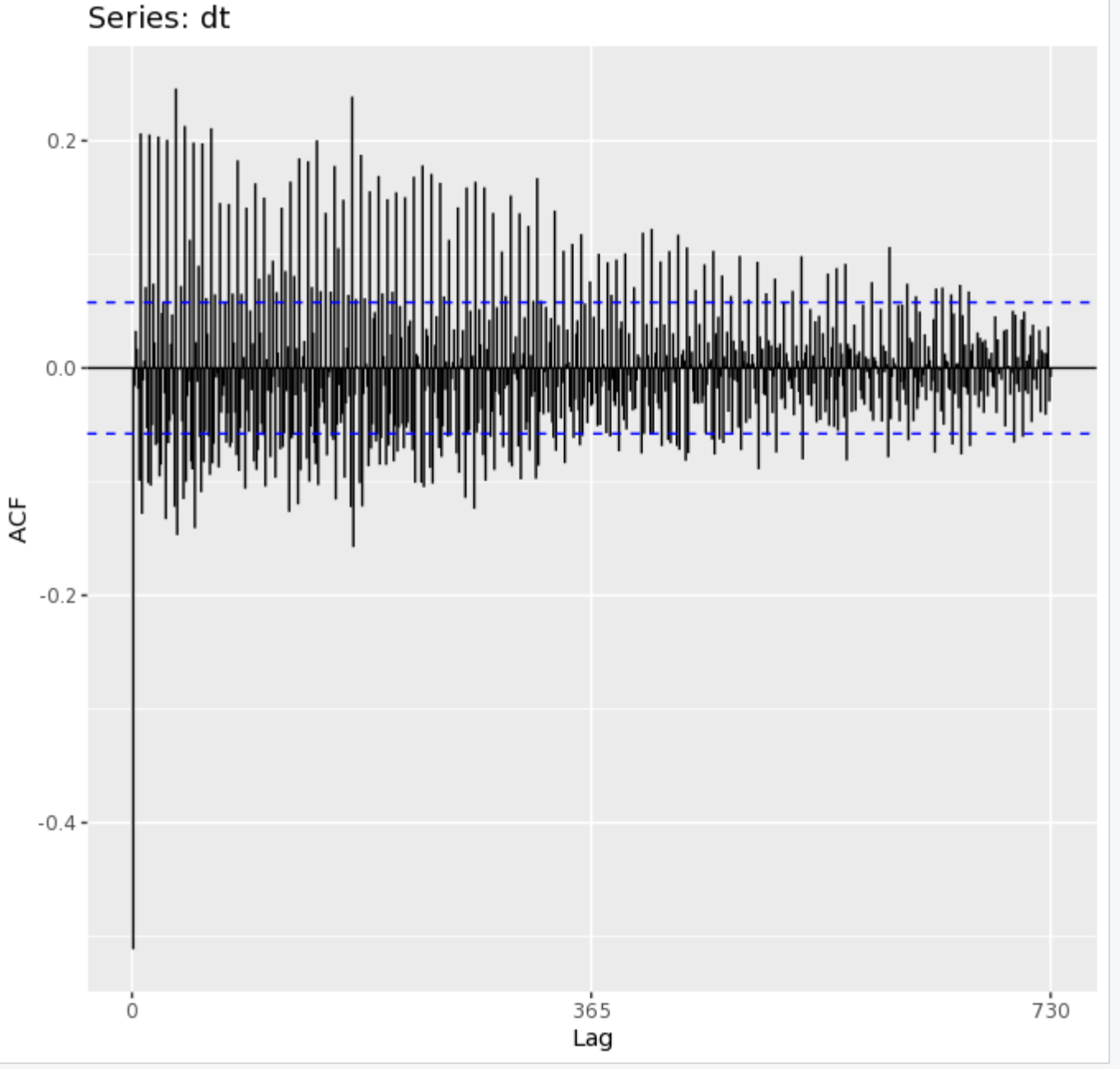
Here's the ACF plot given these transformations -

enter image description here

$\endgroup$
5
  • 1
    $\begingroup$ Your series is not stationary! It clearly shows an upward trend, which makes things quite confusing for study of autocorrelation. I would work on the differenciated series $Y_t:=X_t - X_{t-1}$ rather than on the original $X_t$ If the problem persists, then try $Z_t:=Y_t - Y_{t-1}$ and so on... $\endgroup$
    – David
    Commented May 27, 2019 at 8:28
  • $\begingroup$ I updated the chart. What I'm seeing is that there is a strong positive correlation at a consistent interval, a strong negative correlation at a consistent interval and a few weeker effect too. My data is daily ecommerce revenue. Does this suggest to you that the effect is a function of the day of the week? $\endgroup$
    – ivan
    Commented May 27, 2019 at 15:39
  • 1
    $\begingroup$ the series are not only nonstationary on mean, but the variance seems increasing too. you cant apply ACF/PACF analysis until you address mean and variance instability, e.g. by log differencing $\endgroup$
    – Aksakal
    Commented May 27, 2019 at 15:39
  • $\begingroup$ @Aksakal Do you think that that increase in variance as time goes on has to do with the fact that the original series was also growing? I mean, we'd have something like a constant coefficient of variation, but not constant variance. Because in that case maybe the series to work with is the "return" series $Y_t:=(X_t−X_{t−1})/X_{t-1}$ $\endgroup$
    – David
    Commented May 27, 2019 at 15:48
  • 1
    $\begingroup$ @David, it very well can be. The log differencing (continuous return) is similar to simple return that you refer to in this respect. It doesn't have to be the log rule though, it can be power law. $\endgroup$
    – Aksakal
    Commented May 27, 2019 at 15:50

1 Answer 1

1
$\begingroup$

Power transforms suggested by the error variance being linked to the expected value can be useful Detrending or not and should I always take log first? and here When (and why) should you take the log of a distribution (of numbers)? BUT more often there may be points in the error variance changes deterministically Removing Variance in Time Series After Applying Log Transformation .

Daily data should be modelled (read " generally stay clear of simple 365 period arima stuff " ) when human habits create daily effects, monthly effects , lead and lag effects around holidays , day-of-the-month-effects , week-of-the-month effects . week-of-the-year effects et al. After identifying level shifts and or local time trends then study the residuals for an ARIMA modification.

See https://stats.stackexchange.com/search?tab=newest&q=user%3a3382%20daily for a number of interesting example where daily data is analyzed using a hybrid approach of time effects and memory.

$\endgroup$

Your Answer

By clicking “Post Your Answer”, you agree to our terms of service and acknowledge you have read our privacy policy.

Not the answer you're looking for? Browse other questions tagged or ask your own question.