0
$\begingroup$

I'm trying to reduce highly dimensional data with factor methods. I'm using Principal component analysis and Partial least squares.

From these methods I'm using the first component as a Common factor to summarize the data.

Is it possible that PCA and PLS produce wildly different first components with the same initial data? Or is the R code wrong?

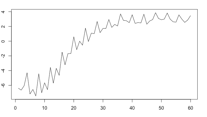
enter image description here

Figure 1: The first Principal component

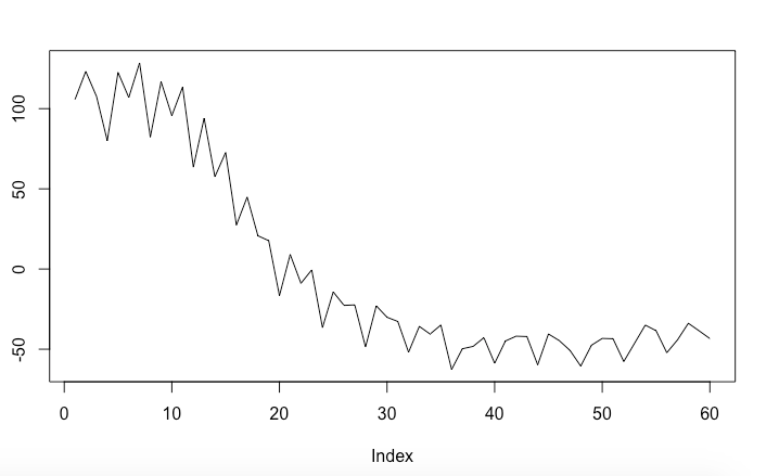
enter image description here

Figure 2: The first PLS component

These figures imply that first components have pretty different kind of trend. Is this normal that first components are so different between the PCA and PLS?

My code for the PLS and PCA were:

#PLS model_pls <- plsr(y ~ as.matrix(X), data = ddata) first_comp_pls<- scores(model_pls)[,1]

#PCA #excluding the y variable newddata <- ddata[2:19] model_pca <- prcomp(newddata, scale =TRUE) first_comp_pca <- model_pca$x[,1]

Thank you for advance!

$\endgroup$

1 Answer 1

1
$\begingroup$

Firstly: it can be that the results of PCA and PLS are different, since they have a different objective function. Especially if the covariance between $X$ and $Y$ is near zero, the PLS solution is not stable.

Secondly: it seems from your plots that you need to multiply the PCA or PLS component with -1. This is allowed, because the sign isn't identifiable anyway. Then, from a visual perspective, they become fairly similar apart from the scale.

And thirdly: it is useful to include code where you define ddata, so that we can actually run the code.

$\endgroup$

Your Answer

By clicking “Post Your Answer”, you agree to our terms of service and acknowledge you have read our privacy policy.

Not the answer you're looking for? Browse other questions tagged or ask your own question.