Background:
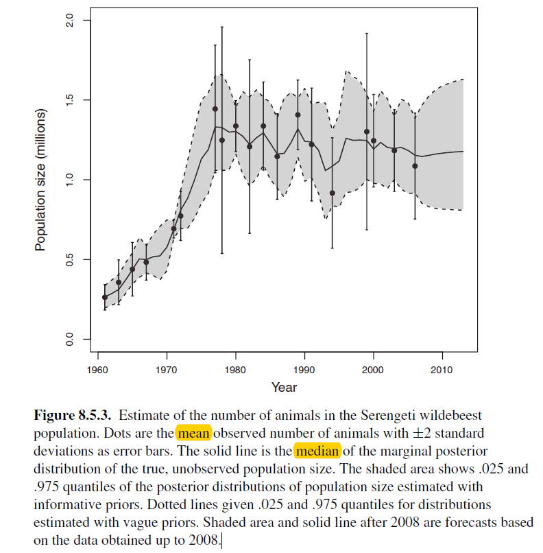
In Chapter8 of this great book, the authors build a Bayesian model and use  to show the posterior distributions of the latent state $N_{t}$ and its credible intervals. The model is written as below:
\begin{aligned} \left[N,\beta,\sigma_p^2|y\right]\propto&\prod normal(y_{t}|N_{t},\sigma_{data,t}^2)\\ \times&\prod lognormal(N_{t}|log(g(\beta,N_{t-1},x_{t})),\sigma_{p}^2))\\ \times &normal(\beta_{0}|0.234,0.0185)\prod_{i=1}^3normal(\beta_{i}|0,100)\\ \times&inverse\ gamma(\sigma_{p}^2|0.01,0.01)\\ \times&normal(N_{1}|y_{1},\sigma_{data,t}^2) \end{aligned}
where: $N_{t}$ is the unobserved, true abundance of wildebeest in year t; $x_{t}$ is a measure of the annual rainfall; $\beta$ is the coefficients; $\sigma_{p}^2$ is the process variance; $\sigma_{data,t}^2$ is a variance for the total population based on the sample of paragraphs.
My questions are:
(1) In Fig.1, why do we compare "mean" observed number of animals with "median" of the marginal posterior distribution of the population size (see the Figure's caption)? Why not use "mean" of the marginal posterior distribution to be consistent with dots (i.e., mean)?
(2) The authors remind us that:
The fit of the model medians is not smooth but, rather, tends to jump a bit between time steps. ... if we assumed that observation variance was 0, such that the true state was exactly the same as the observed state, then the medians would go through every data point.
Then they emphasize that:
It may be counterintuitive that a model like this one that does hit every point, or close to it, is probably not a very good model. What this says is that process variance is high relative to observation variance. The predictive value of such a model will be low.
Why would the solid line go through every data point if the observation variance was 0?
