Why do my splines become not more flexible after altering the parameters in R mgcv?

Question

I have done a logistic regression with two independent variables (x1 and x2) and a dependent binary variable (y). The AUC (roc curve) is 0.7915.

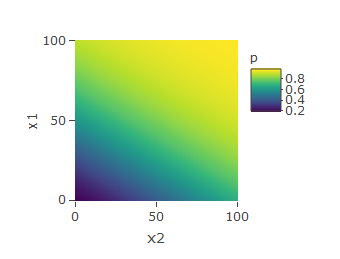
After making a heatmap, I noticed the logistic regression was not flexible enough since the range of y for x1=10 is 0.25 – 0.76 while in reality this range is 0.25 – 1.

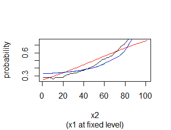
For that reason I have tried to add splines with package mgcv. This results in an improvement. The AUC (roc curve) improves to 0.8069. The improvement is also visible in the graph below.

Red line: logistic regression Blue line: logistic regression with splines, setting sp=0.1 Green line: logistic regression with splines, setting sp=0.9 Black line: Raw data: for every (x1,x2): y=1 / total y

model_1 <- glm(y ~ x2+x1, data = mydata3, family=binomial())
model_2 <- gam(y ~ s(x2, bs="tp", sp=0.1) + s(x1, bs="tp", sp=0.1), data = mydata3, family=binomial())
model_3 <- gam(y ~ s(x2, bs="cr", sp=0.9) + s(x1, bs="cr", sp=0.9), data = mydata3,  family=binomial())
pivot10 <- mydata3 %>% group_by(x1, x2) %>% summarize(mean = mean(y)) %>% filter(x1==10)

It seems to me the logistic regression with splines is still not flexible enough since the black line has more curve than the blue and green lines. I have tried to modify the settings to make the splines more flexible. I have done this by altering the settings for parameter sp. I have also experimented with several types for parameter bs: “ds”, “cr”, “ps” and “te”. Although all these influences are negligible. Illustrative is the small difference between the green and the blue line.

Does someone has solution to make the splines more flexible?

Thank you!

Answer 1

I not sure what you are trying to achieve by setting the smoothness parameter of the smooth function directly. If you are simply trying to fix the wiggliness of the smooth at some value then you would be better off fixing the effective degrees of freedom (EDF) of the smooth by setting k to the required value and also using fx = TRUE in the definition of the smooth.

Note that the EDF of the smooth is equal to k - 1 because one basis function is removed from the smooth as it is a constant function and is unidentifiable in a model that also has an intercept.

gam(y ~ s(x2, bs="tp", k = 15, fx = TRUE) + 
      s(x1, bs="tp", k = 15, fx = TRUE),
    method = 'REML',
    data = mydata3, family=binomial())

In the above code block, we would have a model with two smooths, each of 14 effective degrees of freedom, with fitting done using REML.

Unless you have very good reason to do this however, I would be very careful how you interpret such a model. Normally, one would just set k to be large enough, which can be checked using gam.check() and let the wiggliness penalty decide how complex the estimated smooth functions should be. Otherwise you could be badly under or over-fitting the data and not know it.

As to the specific question, I think you'd need to vary the smoothness parameter over much larger ranges to get the desired effect. This isn't a value that should be in the range 0–1, instead it should be some value in the range 0–∞, with 0 being no wiggliness penalty (hence the full wiggliness implied by EDF == k - 1), and ∞ meaning a purely linear fit (on the link scale).