First, consider just the control group. Suppose you want to see if there
is a difference between baseline and post-treatment. If data are nearly normal
and you have more than just a few subjects, then you can do a 'paired' t test.
(This amounts to doing a one-sample t test on the 'post minus pre; differences.)
For example, if you have $n = 30$ subjects, then 'pre' and 'post' scores
might be as follows:
      [,1]  [,2]  [,3]  [,4]  [,5]  [,6]  [,7]  [,8]  [,9] [,10]
pre  50.71 52.64 53.12 56.73 53.56 46.60 52.03 55.22 52.44 50.34
post 54.07 58.28 58.33 62.01 58.18 53.11 55.89 61.29 57.32 55.76
     [,11] [,12] [,13] [,14] [,15] [,16] [,17] [,18] [,19] [,20]
pre  55.09 43.46 49.27 48.88 47.27 47.57 49.59 47.78 50.42 54.89
post 59.41 47.69 53.09 53.26 50.92 52.31 54.66 52.92 57.05 60.20
     [,21] [,22] [,23] [,24] [,25] [,26] [,27] [,28] [,29] [,30]
pre  54.00 48.46 48.40 50.63 50.12 54.25 52.85 46.45 54.66 49.67
post 59.78 53.40 54.89 54.18 55.81 61.07 58.16 51.72 59.09 54.50
Then summaries and improvement scores imp from R would be as follows:
summary(pre); sd(pre)
   Min. 1st Qu.  Median    Mean 3rd Qu.    Max.
  43.46   48.56   50.52   50.90   53.45   56.73
[1] 3.18757
summary(post); sd(post)
   Min. 1st Qu.  Median    Mean 3rd Qu.    Max.
  47.69   53.30   55.78   55.95   58.32   62.01
[1] 3.451662
imp = post - pre
summary(imp); sd(imp)
   Min. 1st Qu.  Median    Mean 3rd Qu.    Max.
  3.360   4.393   5.105   5.042   5.585   6.820
[1] 0.9280126
We wish to test $H_0: \mu_2 = \mu_1$ against $H_a: \mu_2 > \mu_1.$ In R, a one-sided, paired t test can be done in either of two ways. Full results
are shown for the first. The second method uses t.test(imp, alt="gr"), giving essentially the same result. Because the P-value is essentially equal to $0$ the difference is significant at the 5% level, the 1% level, and any other
reasonable significance level.
t.test(post, pre, pair=T, alt="gr")

        Paired t-test

data:  post and pre
t = 29.756, df = 29, p-value < 2.2e-16
alternative hypothesis: true difference in means is greater than 0
95 percent confidence interval:
 4.753782      Inf
sample estimates:
mean of the differences
               5.041667
Second, if you want to see whether improvement scores are different between
treatment and control groups, you would do a two-sample t test. I have no idea what TAU is, but I assume there is a similar improvement scor, which we might call 'imp.c'.
imp.c
 [1] 4.57 2.76 3.74 5.41 6.71 4.85 4.85 4.87 5.17 5.77
[11] 3.13 3.11 3.96 3.36 4.35 3.74 4.07 5.86 5.81 5.16
[21] 4.90 5.33 4.13 5.02 2.33 3.81 3.01 3.17 3.94 4.65
summary(imp.c); sd(imp.c)
   Min. 1st Qu.  Median    Mean 3rd Qu.    Max.
  2.330   3.740   4.460   4.385   5.125   6.710
[1] 1.055687
Because it is reasonable to suppose that imp and imp.c may come
from populations with different variances, it is best to use a Welch
two-sample test. Also, it seems best to do a two-sided test because
the purpose of the study is to see whether the treatment method differs
from the control. There is a significant difference at the 5% level,
but not (quite) at the 1% level.
t.test(imp, imp.c)

        Welch Two Sample t-test

data:  imp and imp.c
t = 2.5602, df = 57.062, p-value = 0.01313
 alternative hypothesis: true difference in means is not equal to 0
95 percent confidence interval:
 0.1431308 1.1708692
sample estimates:
mean of x mean of y
 5.041667  4.384667
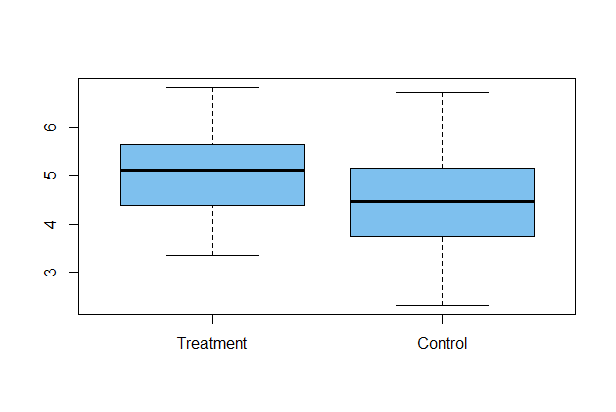
Here are boxplots of improvement scores:
boxplot(imp, imp.c, col="skyblue2", names=c("Treatment","Control"))

Note: If data seem far from normal, you might want to use a nonparametric one-sample Wilcoxon Signed-Rank test to judge whether
improvement scores are significantly above $0,$ and a nonparametric
two-sample Wilcoxon Rank-Sum test to judge whether Treatment and Control scores differ.

