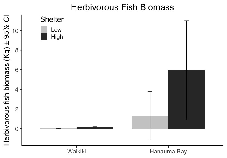
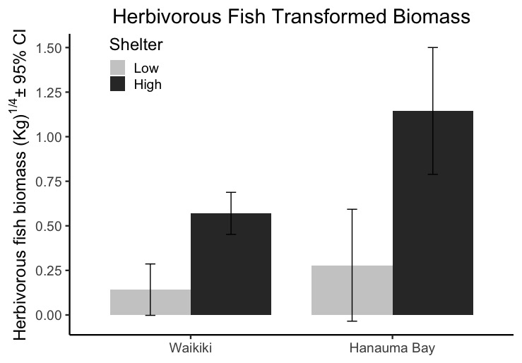
In order to determine how herbivorous fish biomass varies between the two study sites (Waikiki and Hanauma Bay) and experimental shelter treatments (low and high), I used lmer() with a random effect for module (6 at each site) to account for repeated measures through time. Because these data are zero-inflated and continuous in nature, I transformed biomass (total_biomass^(1/4)).
Database
library(lme4)
library(rcompanion)
library(emmeans)

z <- structure(list(Date = structure(c(1L, 1L, 1L, 1L, 1L, 1L, 2L,
2L, 2L, 2L, 2L, 2L, 3L, 3L, 3L, 3L, 3L, 3L, 4L, 4L, 4L, 4L, 4L,
4L, 5L, 5L, 5L, 5L, 5L, 5L, 6L, 6L, 6L, 6L, 6L, 6L, 7L, 7L, 7L,
7L, 7L, 7L, 8L, 8L, 8L, 8L, 8L, 8L), .Label = c("11/28/17", "12/3/17",
"5/15/18", "5/20/18", "5/25/17", "6/6/17", "9/5/17", "9/7/17"
), class = "factor"), `Module #` = c(211L, 212L, 213L, 214L,
215L, 216L, 111L, 112L, 113L, 114L, 115L, 116L, 211L, 212L, 213L,
214L, 215L, 216L, 111L, 112L, 113L, 114L, 115L, 116L, 111L, 112L,
113L, 114L, 115L, 116L, 211L, 212L, 213L, 214L, 215L, 216L, 211L,
212L, 213L, 214L, 215L, 216L, 111L, 112L, 113L, 114L, 115L, 116L
), Site_long = structure(c(1L, 1L, 1L, 1L, 1L, 1L, 2L, 2L, 2L,
2L, 2L, 2L, 1L, 1L, 1L, 1L, 1L, 1L, 2L, 2L, 2L, 2L, 2L, 2L, 2L,
2L, 2L, 2L, 2L, 2L, 1L, 1L, 1L, 1L, 1L, 1L, 1L, 1L, 1L, 1L, 1L,
1L, 2L, 2L, 2L, 2L, 2L, 2L), .Label = c("Hanauma Bay", "Waikiki"
), class = "factor"), Treatment_long = structure(c(2L, 1L, 2L,
1L, 2L, 1L, 2L, 1L, 2L, 1L, 2L, 1L, 2L, 1L, 2L, 1L, 2L, 1L, 2L,
1L, 2L, 1L, 2L, 1L, 2L, 1L, 2L, 1L, 2L, 1L, 2L, 1L, 2L, 1L, 2L,
1L, 2L, 1L, 2L, 1L, 2L, 1L, 2L, 1L, 2L, 1L, 2L, 1L), .Label = c("Closed",
"Open"), class = "factor"), Shelter = structure(c(1L, 2L, 1L,
2L, 1L, 2L, 1L, 2L, 1L, 2L, 1L, 2L, 1L, 2L, 1L, 2L, 1L, 2L, 1L,
2L, 1L, 2L, 1L, 2L, 1L, 2L, 1L, 2L, 1L, 2L, 1L, 2L, 1L, 2L, 1L,
2L, 1L, 2L, 1L, 2L, 1L, 2L, 1L, 2L, 1L, 2L, 1L, 2L), .Label = c("High",
"Low"), class = "factor"), TimeStep = c(5L, 5L, 5L, 5L, 5L, 5L,
5L, 5L, 5L, 5L, 5L, 5L, 7L, 7L, 7L, 7L, 7L, 7L, 7L, 7L, 7L, 7L,
7L, 7L, 1L, 1L, 1L, 1L, 1L, 1L, 1L, 1L, 1L, 1L, 1L, 1L, 4L, 4L,
4L, 4L, 4L, 4L, 4L, 4L, 4L, 4L, 4L, 4L), total_biomass = c(0.0526394784788566,
0.00650991088549517, 0.180596698411345, 0, 0.526717015131238,
0, 0.209199851062596, 0, 0.283172330030785, 0, 0.394899281159044,
0.176129136061979, 10.6461511880577, 0, 26.4504921170652, 0,
0.526717015131238, 0, 0, 0, 0.403061371653634, 0.209695276260751,
0.120034320302602, 0.0206199419933497, 0.078489026854395, 0,
0.165344302422082, 0, 0.0317487117533543, 0, 0.169586003898729,
0.125258604363503, 0.35499517850828, 0, 10.6461511880577, 0,
0.35257770725851, 0.0520989800170256, 0.222619650542138, 0, 21.2935111117403,
15.7227719241434, 0.232861857335555, 0, 0.0634974235067086, 0,
0.0492074004365164, 0), new_date = structure(c(17498, 17498,
17498, 17498, 17498, 17498, 17503, 17503, 17503, 17503, 17503,
17503, 17666, 17666, 17666, 17666, 17666, 17666, 17671, 17671,
17671, 17671, 17671, 17671, 17311, 17311, 17311, 17311, 17311,
17311, 17323, 17323, 17323, 17323, 17323, 17323, 17414, 17414,
17414, 17414, 17414, 17414, 17416, 17416, 17416, 17416, 17416,
17416), class = "Date"), biomass_trans = c(0.478991596851473,
0.284049324543866, 0.651894702163611, 0, 0.851911217868642, 0,
0.676301487671506, 0, 0.729478847988674, 0, 0.79272323151449,
0.647825145430307, 1.80633441911244, 0, 2.26781925907219, 0,
0.851911217868642, 0, 0, 0, 0.796788018050487, 0.676701535344577,
0.58860826961759, 0.378941229433868, 0.52930041698453, 0, 0.637671942584471,
0, 0.422115720944064, 0, 0.641722847123095, 0.594910853348915,
0.771890353787985, 0, 1.80633441911244, 0, 0.770572866160467,
0.477757270887696, 0.686895820978435, 0, 2.14813622890879, 1.99127975623794,
0.694663674551471, 0, 0.501983018701184, 0, 0.470985574485205,
0)), class = c("grouped_df", "tbl_df", "tbl", "data.frame"), row.names = c(NA,
-48L), vars = c("Date", "Module #", "Site_long", "Treatment_long",
"Shelter"), labels = structure(list(Date = structure(c(1L, 1L,
1L, 1L, 1L, 1L, 2L, 2L, 2L, 2L, 2L, 2L, 3L, 3L, 3L, 3L, 3L, 3L,
4L, 4L, 4L, 4L, 4L, 4L, 5L, 5L, 5L, 5L, 5L, 5L, 6L, 6L, 6L, 6L,
6L, 6L, 7L, 7L, 7L, 7L, 7L, 7L, 8L, 8L, 8L, 8L, 8L, 8L), .Label = c("11/28/17",
"12/3/17", "5/15/18", "5/20/18", "5/25/17", "6/6/17", "9/5/17",
"9/7/17"), class = "factor"), `Module #` = c(211L, 212L, 213L,
214L, 215L, 216L, 111L, 112L, 113L, 114L, 115L, 116L, 211L, 212L,
213L, 214L, 215L, 216L, 111L, 112L, 113L, 114L, 115L, 116L, 111L,
112L, 113L, 114L, 115L, 116L, 211L, 212L, 213L, 214L, 215L, 216L,
211L, 212L, 213L, 214L, 215L, 216L, 111L, 112L, 113L, 114L, 115L,
116L), Site_long = structure(c(1L, 1L, 1L, 1L, 1L, 1L, 2L, 2L,
2L, 2L, 2L, 2L, 1L, 1L, 1L, 1L, 1L, 1L, 2L, 2L, 2L, 2L, 2L, 2L,
2L, 2L, 2L, 2L, 2L, 2L, 1L, 1L, 1L, 1L, 1L, 1L, 1L, 1L, 1L, 1L,
1L, 1L, 2L, 2L, 2L, 2L, 2L, 2L), .Label = c("Hanauma Bay", "Waikiki"
), class = "factor"), Treatment_long = structure(c(2L, 1L, 2L,
1L, 2L, 1L, 2L, 1L, 2L, 1L, 2L, 1L, 2L, 1L, 2L, 1L, 2L, 1L, 2L,
1L, 2L, 1L, 2L, 1L, 2L, 1L, 2L, 1L, 2L, 1L, 2L, 1L, 2L, 1L, 2L,
1L, 2L, 1L, 2L, 1L, 2L, 1L, 2L, 1L, 2L, 1L, 2L, 1L), .Label = c("Closed",
"Open"), class = "factor"), Shelter = structure(c(1L, 2L, 1L,
2L, 1L, 2L, 1L, 2L, 1L, 2L, 1L, 2L, 1L, 2L, 1L, 2L, 1L, 2L, 1L,
2L, 1L, 2L, 1L, 2L, 1L, 2L, 1L, 2L, 1L, 2L, 1L, 2L, 1L, 2L, 1L,
2L, 1L, 2L, 1L, 2L, 1L, 2L, 1L, 2L, 1L, 2L, 1L, 2L), .Label = c("High",
"Low"), class = "factor")), row.names = c(NA, -48L), vars = c("Date",
"Module #", "Site_long", "Treatment_long", "Shelter"), drop = TRUE, class = "data.frame"), indices = list(
    0L, 1L, 2L, 3L, 4L, 5L, 6L, 7L, 8L, 9L, 10L, 11L, 12L, 13L,
    14L, 15L, 16L, 17L, 18L, 19L, 20L, 21L, 22L, 23L, 24L, 25L,
    26L, 27L, 28L, 29L, 30L, 31L, 32L, 33L, 34L, 35L, 36L, 37L,
    38L, 39L, 40L, 41L, 42L, 43L, 44L, 45L, 46L, 47L), drop = TRUE, group_sizes = c(1L,
1L, 1L, 1L, 1L, 1L, 1L, 1L, 1L, 1L, 1L, 1L, 1L, 1L, 1L, 1L, 1L,
1L, 1L, 1L, 1L, 1L, 1L, 1L, 1L, 1L, 1L, 1L, 1L, 1L, 1L, 1L, 1L,
1L, 1L, 1L, 1L, 1L, 1L, 1L, 1L, 1L, 1L, 1L, 1L, 1L, 1L, 1L), biggest_group_size = 1L)
Distribution
plotNormalHistogram(z$total_biomass, main = "Biomass")
plotNormalHistogram(z$biomass_trans, main = "Transformed Biomass")
lmer
# variables
module_fish <- z$`Module #`

## Biomass transformed ##
fish_mixed_effects_trans <- lmer(biomass_trans ~ Site_long*Shelter + (1|module_fish), data = z, na.action = "na.fail")
summary(fish_mixed_effects_trans)

> summary(fish_mixed_effects_trans)
Linear mixed model fit by REML. t-tests use Satterthwaite's method ['lmerModLmerTest']
Formula: biomass_trans ~ Site_long * Shelter + (1 | module_fish)
   Data: mean_fish_totals

REML criterion at convergence: 68.4

Scaled residuals:
    Min      1Q  Median      3Q     Max
-1.4148 -0.5931 -0.3018  0.3598  3.6398

Random effects:
 Groups      Name        Variance Std.Dev.
 module_fish (Intercept) 0.0000   0.0000
 Residual                0.2213   0.4704
Number of obs: 48, groups:  module_fish, 12

Fixed effects:
                            Estimate Std. Error      df t value Pr(>|t|)
(Intercept)                   1.1445     0.1358 44.0000   8.428 9.88e-11 ***
Site_longWaikiki             -0.5745     0.1921 44.0000  -2.991  0.00454 **
ShelterLow                   -0.8655     0.1921 44.0000  -4.507 4.82e-05 ***
Site_longWaikiki:ShelterLow   0.4374     0.2716 44.0000   1.611  0.11442
---
Signif. codes:  0 ‘***’ 0.001 ‘**’ 0.01 ‘*’ 0.05 ‘.’ 0.1 ‘ ’ 1

Correlation of Fixed Effects:
            (Intr) St_lnW ShltrL
Site_lngWkk -0.707
ShelterLow  -0.707  0.500
St_lngWk:SL  0.500 -0.707 -0.707
convergence code: 0
singular fit
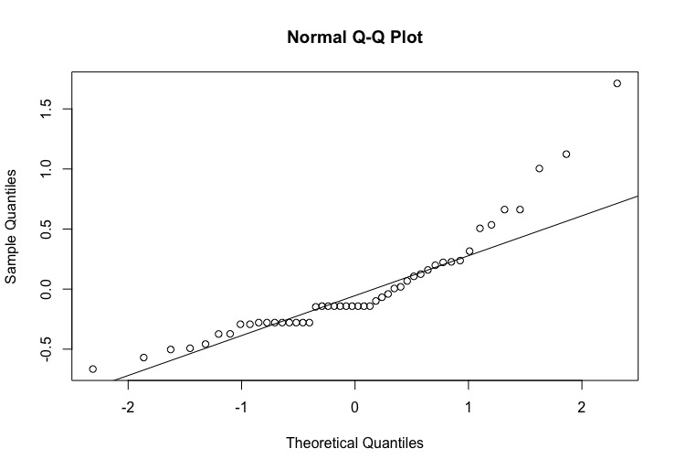
QQplot for Transformed Biomass Analysis
Pairwise Comparison
emm_fish <- emmeans(fish_mixed_effects_trans, ~Site_long*Shelter)
pairs(emm_fish)

> pairs(emm_fish)
 contrast                            estimate        SE df t.ratio p.value
 Hanauma Bay,High - Waikiki,High    0.5744829 0.1920508  8   2.991  0.0673
 Hanauma Bay,High - Hanauma Bay,Low 0.8655348 0.1920508  8   4.507  0.0086
 Hanauma Bay,High - Waikiki,Low     1.0025789 0.1920508  8   5.220  0.0035
 Waikiki,High - Hanauma Bay,Low     0.2910519 0.1920508  8   1.515  0.4721
 Waikiki,High - Waikiki,Low         0.4280960 0.1920508  8   2.229  0.1950
 Hanauma Bay,Low - Waikiki,Low      0.1370441 0.1920508  8   0.714  0.8890

P value adjustment: tukey method for comparing a family of 4 estimates
Considering that both Site_long and Shelter are significant predictors, I assumed that the pairwise comparison from emmeans() would result in significant p-values for "Hanauma Bay,High - Waikiki,High" and "Hanauma Bay,High - Waikiki,Low".
I am attempting to place letters above error bars to signify the results of the pairwise comparison but was confused that the difference between "Hanauma Bay,High - Waikiki,Low" was significant while the "Hanauma Bay,High - Waikiki,High" is not. How should I interpret these results and should I use some other method for pairwise comparisons? Thank you for your time.


