0
$\begingroup$

I'm trying to employ an ARIMA model, and have run into the following conundrum:

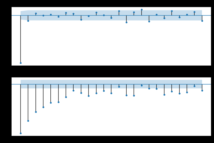
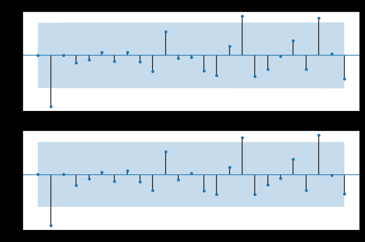
when I employ differencing or other transforms to successfully achieve stationarity (at least according to the Augmented Dickey Fuller Test), my ACF/PACF plots are ambiguous at best:

ACF&PACF Plots

...yet only when I employ a transform that does not achieve stationarity via Dickey Fuller standards (sub-optimal p values of 1-3) am I actually able to obtain typical ACF/PACF plots that could yield the order of my model.

Better plot, worse stationarity

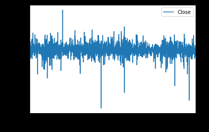
Knowing that Dickey Fuller can only test stationarity with regards to trend (and not variance and other factors), I'm left to wonder if the problem is that my data isn't as stationary as indicated by that test. As you will see from the plot, there are certain considerable outliers, so I considered that they were the root of the problem:

Time Series After Differencing

Yet even after dealing with these outliers in a variety of ways, and improving stationarity as reflected by Dickey Fuller (and a more stationary-looking plot), my ACF/PACF plots remain just as ambiguous as shown in the first figure. I have tried many means of differencing and transforming, but with the same result. Is lack of stationarity still the likely problem? Or is it something else I'm not considering, and if so, what? Thank you in advance.

My data (weekly price data going back to November 2010) can be found here: https://www.dropbox.com/s/gl3irup6csygctf/WBAWeekly.csv?dl=0

$\endgroup$
10
  • $\begingroup$ What do you mean your ARIMA is failing? In what way? In that it does not achieve stationarity in the residuals? Have you tried different terms of AR and MA? $\endgroup$ Commented Aug 8, 2019 at 6:07
  • 1
    $\begingroup$ post your data and I will try and help. $\endgroup$
    – IrishStat
    Commented Aug 8, 2019 at 7:11
  • $\begingroup$ @user2974951- it's not that the ARIMA is failing per se, it's that my ARIMA modeling process is failing in that I can't transform my data such that it can plot the kind of ACF/PACF from which I could derive my model order. $\endgroup$
    – pmse234
    Commented Aug 8, 2019 at 12:55
  • $\begingroup$ @IrishStat thank you! I have seen your other posts and had hoped you would notice my thread. I’ve updated my post with a link to my data. $\endgroup$
    – pmse234
    Commented Aug 9, 2019 at 0:01
  • $\begingroup$ OK .. it appears that your are missing days such as xmas and xms eve et al . Time series analysis requires an observation for every day . please interpolate to get missing values and repost.. $\endgroup$
    – IrishStat
    Commented Aug 9, 2019 at 2:00

1 Answer 1

0
$\begingroup$

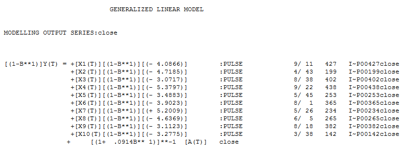
I took your weekly data enter image description here and developed a model that was essentially a random walk with some anomalies enter image description here .

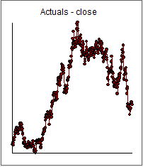
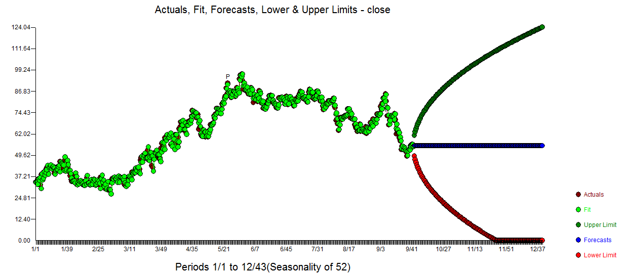
The Actual,Fit and Forecast is here enter image description here

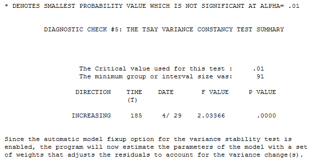
The developed model required GLS essentially using weights to stabilize the error variance per here enter image description here . The Error variance is visually larger starting around week 185 .

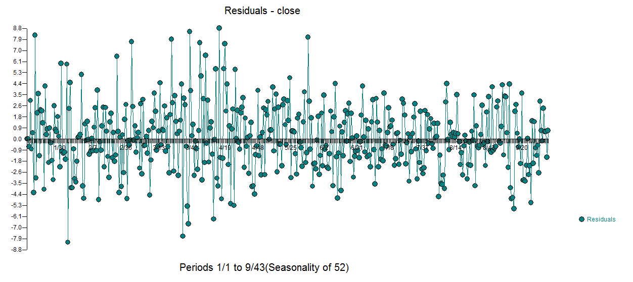
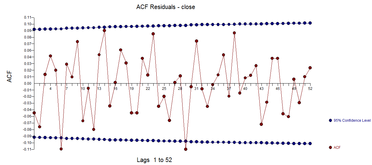
The final plot of errors appears random enter image description here with an ACF here enter image description here

Fama suggested many moons ago that the stock market was a random walk and this of course is applicable to all the speculative price markets.

$\endgroup$
7
  • $\begingroup$ Very interesting, thank you- to develop my intuition, I suppose the answer to my original question is that the reason the (p)acf plots were ambiguous and inadequate for ARIMA modeling is not due to lack of stationarity, but because a Random Walk model is more explanatory of the price movement than one of the ARIMA variety? If I have that right, does that mean modeling price data with ARIMA means having to forego using ambigous acf/pacf plots as a means of choosing model order, perhaps to use other means like AIC/BIC? Thank you $\endgroup$
    – pmse234
    Commented Aug 11, 2019 at 7:10
  • $\begingroup$ autobox.com/pdfs/ARIMA%20FLOW%20CHART.pdf a random walk model is an ARIMA model (0,1,0)(),0,0) if the error variance is homogeneous through time AND there are no pulses,step/level shifts, seasonal pulses,local time trends. You can't upvote my answer but you can accept it. $\endgroup$
    – IrishStat
    Commented Aug 11, 2019 at 11:34
  • $\begingroup$ Thank you! I suppose then, in the context of the original question, it’s not that my ambiguous (p)acf plots are indicative of a failing model, but that they are reflective of ARIMA modeling indicating a random walk. Also, I had seen your pdf flowchart before originally posting and wondered if I was interpreting it correctly: it seems it would entail using AIC/BIC over eyeballing the plots anyway, right? $\endgroup$
    – pmse234
    Commented Aug 13, 2019 at 13:27
  • $\begingroup$ Your ambiguous (p)acf plots are a result of the impact of 1) anomalies ; 2) error variance changing at 1 deterministic point in time .... it is not the fault of the underlying ARIMA structure. The AIC of a bad model is always flawed to one degree or another and thus is NOTt the robust way of identifying a model ..JUST A WAY OF JUDGING A PRESUMED SET OF MODELS.. Your data suggests the need for the two remedies 1) pulse deterministic structure & 2 ) Generalize least squares (Weighted Least Squares in this case) $\endgroup$
    – IrishStat
    Commented Aug 13, 2019 at 13:48
  • $\begingroup$ To address the first of the proposed remedies, I see in this thread with a seemingly similar issue you refer the poster to a paper by Tsay: stats.stackexchange.com/questions/384502/…. Is that where I can best learn to apply these remedies myself? And as for the GLS, I see in the model output you posted above, it mentions Tsay- does that same paper address the second remedy (GLS) too? If not, would you kindly point me to the right resources? Thank you for your help! $\endgroup$
    – pmse234
    Commented Aug 13, 2019 at 16:35

Not the answer you're looking for? Browse other questions tagged or ask your own question.